Every statistics course starts the way news articles start: with a claim — “Students who sleep less report more stress,” or “Coffee drinkers live longer.” Before you trust a claim like that, you need to ask a few plain questions: Who got measured? How were they chosen? Did anyone do anything to them, or did we just watch and record? This week builds the vocabulary for asking those questions automatically, using a foot-length dataset, a made-up dorm full of sleepy students, and a shelter full of cats.
This week has a lot of new vocabulary — that’s normal
You only need the four goals in the box above by the end of the week; everything else in this unit is here to build toward them. If you would rather read in two shorter sittings, “Cases, variables, and what kind of data is it?” through “Population vs. sample; parameter vs. statistic” make a natural first stop, and “Sampling methods and bias” through “Observational studies vs. experiments” can wait for a second sitting. Every new term is defined the moment it first appears and collected again in Key terms at the end, so you never have to hold a definition in your head — you can always scroll back and check.
1Cases, variables, and what kind of data is it?
Every dataset you meet this semester is, underneath, a table. Each case (also called an observation) is one row — one kid, one cat, one student. Each variable is one column — a characteristic that can differ from case to case. Once you’ve found a variable, ask what kind it is, because that decision drives every graph and every formula you’ll use on it later. A numerical (quantitative) variable takes number values you can meaningfully average; it is either discrete (something you count, like a number of pets) or continuous (something you measure on a scale, like a length in centimeters). A categorical (qualitative) variable sorts a case into a group; it is either nominal (the categories have no natural order, like a dominant hand) or ordinal (the categories do have a natural order, like class standing).
Worked example 1. The KidsFeet dataset (package mosaicData) records foot
measurements for children — a real, published teaching dataset, not a
simulation. Here is R peeking at it the way you always should before doing anything
else:
library(mosaic)
nrow(KidsFeet)
names(KidsFeet)
head(KidsFeet)
Table 1. First 6 of 39 rows of KidsFeet.
| name | birthmonth | birthyear | length | width | sex | biggerfoot | domhand |
|---|---|---|---|---|---|---|---|
| David | 5 | 88 | 24.4 | 8.4 | B | L | R |
| Lars | 10 | 87 | 25.4 | 8.8 | B | L | L |
| Zach | 12 | 87 | 24.5 | 9.7 | B | R | R |
| Josh | 1 | 88 | 25.2 | 9.8 | B | L | R |
| Lang | 2 | 88 | 25.1 | 8.9 | B | L | R |
| Scotty | 3 | 88 | 25.7 | 9.7 | B | R | R |
length and width are numerical continuous — measured foot dimensions in
centimeters that can fall anywhere on a scale. sex, domhand, and biggerfoot are
categorical nominal — labels like “B”/“G” or “L”/“R” with no natural ranking.
birthmonth is full of digits (1–12), but it behaves like a category here: nobody’s
month 9 is “more” than month 3, and averaging birth months would mean nothing. That is a
common trap — a column of numbers is not automatically a numerical variable. Ask
yourself: would averaging this number mean anything? If not, it is categorical, even
when it is stored as digits.
2Population vs. sample; parameter vs. statistic
A population is the entire group you actually want to learn about — every CSUB student, every cat that has ever lived at a shelter. A sample is the subset you actually observe. Because measuring an entire population is rarely possible, we use the sample to estimate facts about the population. A parameter is a numerical summary of the population — a fixed number, usually unknown in real research, written with a Greek letter such as (population mean, “mu”). A statistic is a numerical summary of a sample — a number you actually compute from data, written with a Roman letter such as (sample mean, “x-bar”). A statistic estimates a parameter, but a single sample almost never lands on the parameter exactly; that gap is ordinary sampling variability, an idea we build precise tools for starting in Week 9.
Worked example 2. To see the difference between a parameter and a statistic, we
need a case where we secretly know the whole population — something that never happens
with real data, so we built one on purpose. campus_sleep_sim is a clearly labeled
simulation (the _sim in its name is a signal, not real data) of
students’ nightly sleep hours; 35% of the simulated population has an 8 a.m. class
(early_class), and by design those students sleep somewhat less.
How we built this teaching population, and drew a sample from it (optional)
You do not need to read this box to follow the example — R stays optional all course long,
and this is the one spot all week where the code gets technical. It’s here only for the
curious: rep() repeats a value a set number of times, rnorm() draws random values shaped
like a bell curve (Week 5 explains that shape), and set.seed() makes the “random” numbers
come out the same way every time this code runs, so the results below are always exactly
reproducible.
suppressMessages({library(mosaic); library(BSDA)})
set.seed(1209)
N <- 3000
early_class <- c(rep(TRUE, 1050), rep(FALSE, 1950))
sleep_hours <- c(rnorm(1050, mean = 6.1, sd = 1.0),   # early-class students
                  rnorm(1950, mean = 7.1, sd = 1.0))   # everyone else
campus_sleep_sim <- data.frame(student_id = 1:N, early_class, sleep_hours)

# an honest simple random sample of 40 students
idx <- sample(1:N, size = 40, replace = FALSE)
srs <- campus_sleep_sim[idx, ]
Once the population exists, finding its mean takes R one line:
mean(~sleep_hours, data = campus_sleep_sim) # the population parameter, mu[1] 6.75Across all 3,000 simulated students, the population parameter is hours (population SD hours) — a number we can know exactly only because we built the entire population ourselves. Now find the mean of the honest random sample of students drawn in the box above:
mean(~sleep_hours, data = srs) # the sample statistic, x-bar[1] 6.43This sample’s statistic is hours — close to , but not identical. That is expected: a different random draw of 40 students would give a slightly different every time, even though never moves. Figure 1, just below, compares this honest random sample to a much less trustworthy way of sampling, covered next.
3Sampling methods and bias
How you choose a sample matters as much as how big it is. A simple random sample
(SRS) gives every possible group of cases an equal chance of being picked — in
practice, you assign everyone an ID and let a computer draw at random, exactly like the
sample() call above. A stratified sample first splits the population into
subgroups (strata) that are similar inside themselves — say, class standing — and
then draws a separate random sample from each stratum, guaranteeing every stratum is
represented. A cluster sample instead splits the population into naturally
occurring groups (clusters) — say, discussion sections — randomly selects a handful
of whole clusters, and surveys everyone inside them. All three are legitimate random
sampling methods. A convenience sample — surveying whoever is easiest to reach — is
not: it produces bias, a systematic tendency to miss part of the population that
does not shrink no matter how many people you add.
Worked example 3. Suppose instead of a random draw, a researcher only surveys the first 40 simulated students already sitting in an 8 a.m. class — an easy-to-reach, but non-random, group.
How we picked this convenience sample (optional)
convenience <- campus_sleep_sim[campus_sleep_sim$early_class == TRUE, ][1:40, ]In plain language: take every simulated student with an 8 a.m. class, then keep only the
first 40 of them. That is convenience sampling — grab whoever is easy to reach and stop,
instead of giving everyone an equal chance the way sample() did in the box above.
mean(~sleep_hours, data = convenience)[1] 6.19This convenience sample gives hours — noticeably below the true population mean of 6.75 hours, and even a bit below the honest SRS estimate of 6.43. The problem is not the sample size (both samples have ); it is who is in the sample. Every early-class student we could ever survey belongs to the low-sleep subgroup (subgroup population mean about 6.10 hours), so this method keeps under-estimating no matter how many early-class students we add — that is what makes it biased, not just unlucky. Figure 1, just below, puts all three numbers side by side.
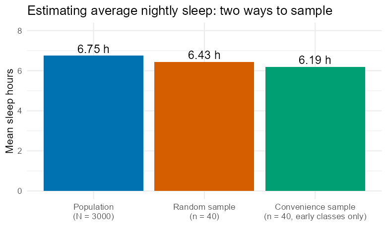
Figure 1. The honest random sample (6.43 h) lands close to the true population mean (6.75 h). The convenience sample of only early-class students (6.19 h) systematically undershoots it — that gap is bias, not bad luck, because it would not close with a bigger convenience sample.
Table 2. Six students from the honest random sample (srs).
| student_id | early_class | sleep_hours |
|---|---|---|
| 2354 | FALSE | 6.45 |
| 569 | TRUE | 8.24 |
| 2951 | FALSE | 6.41 |
| 2020 | FALSE | 6.23 |
| 1664 | FALSE | 7.57 |
| 390 | TRUE | 4.04 |
4Observational studies vs. experiments
A study is observational when researchers measure what is already happening, without assigning anyone to a group — subjects sort themselves. A study is an experiment when researchers deliberately assign each subject to a treatment and compare the outcomes. The variable that might explain a difference is the explanatory variable; the outcome you measure is the response variable.
Here is the rule that drives the rest of the semester: an observational study can show only association, no matter how large it is. Something else might be the real explanation — a confounding variable (also called a lurking variable): something tangled up with both the explanatory and response variable. Only random assignment can rule that out. Random assignment means flipping a coin to decide who gets which treatment. It works because randomization tends to spread every confounding variable evenly across every treatment group, so no group starts out systematically different from another. (Random assignment is a different job from random sampling: sampling is about who is in your study; assignment is about which group each subject lands in.)
In human research, experiments often add a control group — a group given no treatment, or the standard one, for comparison. Some experiments also use a placebo, a fake treatment that looks real. Researchers combine this with blinding: keeping subjects, and sometimes researchers too, unaware of who received which treatment. Both tools rule out explanations other than the treatment itself.
Worked example 4. A shelter’s staff informally — not randomly — give extra
playtime mostly to livelier kittens. shelter_naps_sim is a seeded simulation of 40
cats (20 kittens, 20 adults) in which nap hours depend only on age; by construction,
playtime has no real effect on napping. Compare the groups anyway:
mean(nap_hours ~ extra_playtime, data = shelter_naps_sim) FALSE TRUE
12.62805 15.14084Cats with extra playtime napped 15.14 hours on average versus 12.63 for cats without — a 2.51-hour gap that looks like a real effect of playtime. But check who is actually in each group:
tally(age_group ~ extra_playtime, data = shelter_naps_sim, format = "proportion") extra_playtime
age_group FALSE TRUE
adult 0.778 0.273
kitten 0.222 0.727The extra-playtime group is 72.7% kittens; the no-extra-playtime group is only 22.2% kittens — and kittens simply nap more than adult cats, regardless of playtime. Age is the confounding variable: it is tangled up with both who got playtime and how much each cat napped, so the naive comparison is misleading. Now randomly reassign playtime with a coin flip, completely unrelated to age, and compare the same 40 cats’ same nap hours again:
mean(nap_hours ~ extra_playtime, data = shelter_naps_exp) FALSE TRUE
14.44166 13.48260The apparent gap shrinks from 2.51 hours to 0.96 hours — and flips direction — once random assignment breaks the tie between playtime and age (now 38.9%/61.1% kitten split versus 59.1%/40.9%, much closer to even than the observational 72.7%/22.2%). Nothing about the cats changed; only how the groups were formed changed. That is exactly why “coffee drinkers live longer” headlines deserve the same skepticism: coffee drinkers are not a random sample of everyone, so any health difference might trace back to a confounding variable — like a typical daily routine — rather than the coffee itself. Only a randomized experiment could tell coffee’s effect apart from its confounds.
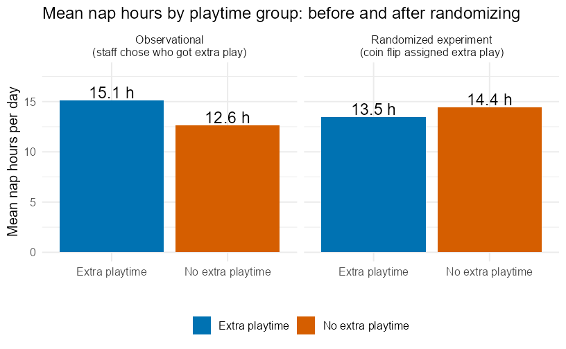
Figure 2. The 2.5-hour gap in the observational comparison shrinks to under one hour — and flips direction — once random assignment decouples playtime from the true confounding variable, age.
5Check your understanding
In the
KidsFeetdata, iswidthnumerical or categorical? If numerical, is it discrete or continuous? Isdomhandnumerical or categorical? If categorical, is it nominal or ordinal?A campus dining survey records (a) the number of energy drinks a student bought this week and (b) their favorite meal (breakfast, lunch, or dinner). Classify each variable.
In Worked example 2 (
campus_sleep_sim), identify the population, the sample, the parameter, and the statistic — including their numeric values.A student wants to know how CSUB students feel about the new dining hall, so she asks the first 20 people she sees in the library. What kind of sample is this, and why might it be biased?
A registrar assigns every one of CSUB’s roughly 7,000 undergraduates a unique ID number, and a computer randomly draws 200 of those IDs to survey. What sampling method is this?
A campus news story claims “students who use the Ask-the-Tutor chatbot earn higher exam scores,” based on comparing students who chose to use it against students who did not. Is this an observational study or an experiment? Can the article fairly claim the chatbot caused higher scores? Explain, naming a possible confounding variable.
6Key terms
population — the entire group a study wants to learn about.
sample — the subset of the population actually observed.
parameter — a numerical summary of a population (usually unknown); Greek letters, e.g. .
statistic — a numerical summary of a sample, computed from data; Roman letters, e.g. .
case (observation) — one row of a data table; one individual or unit.
variable — one column of a data table; a characteristic that can vary case to case.
numerical (quantitative) variable — takes values you can meaningfully average; discrete (counted) or continuous (measured on a scale).
categorical (qualitative) variable — sorts cases into groups; nominal (no natural order) or ordinal (natural order).
explanatory variable / response variable — the possible cause, and the outcome it might explain.
simple random sample (SRS) — every possible sample of size has an equal chance of selection.
stratified sample — random sampling done separately within predefined subgroups (strata).
cluster sample — randomly selected whole groups (clusters), with every member of a chosen cluster included.
bias — a sampling method’s systematic tendency to miss the true population value; does not shrink with a bigger sample.
observational study — subjects are measured, not assigned, to groups.
experiment — researchers deliberately assign subjects to treatments.
treatment / control group — the condition applied to a group; a group given no treatment (or a standard one) for comparison.
placebo / blinding — a fake treatment that looks real; keeping subjects (and sometimes researchers) unaware of who received which treatment.
random assignment — randomly deciding which treatment each subject receives; distinct from random sampling.
confounding variable — a variable tangled up with both the explanatory and response variable, clouding a causal read.