Week 2 — Summarizing Data — Numbers - Statistics in the Modern World (MATH 1209)

A local animal shelter tracks how long each cat naps during the slow afternoon hours — partly for fun, partly because a cat who won’t settle down is harder to place with a family. Staff watched 20 cats one afternoon and logged each nap in hours. Some numbers are unremarkable — a little over an hour, a couple hours, four hours. Two cats, though, barely woke up: one napped almost 9 hours, another over 10. If a volunteer asks “so how long does a cat nap here, typically?” — what’s the honest answer? This week gives you the tools to answer that kind of question for any batch of numbers: a single best “typical” value, a way to describe how spread out the values are, and a way to tell when one or two values don’t behave like the rest.

1Measures of center — mean, median, and mode¶

When you’re staring at 20 numbers, the first thing you want is a single value that stands in for “typical.” There are three common choices, and they don’t always agree.

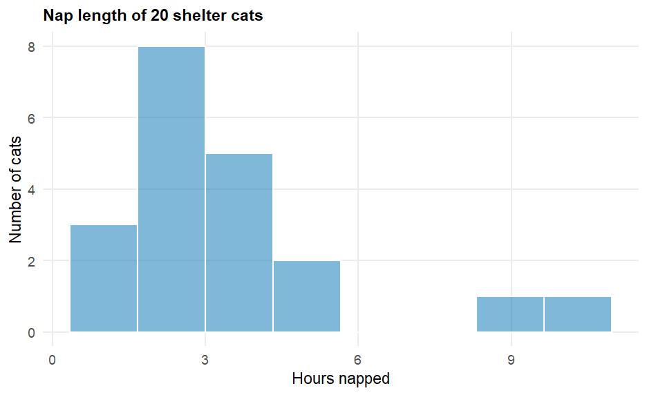
A histogram of the 20 cats' nap lengths shows most bars clustered between 1 and 5 hours, tallest around 2 hours, then a gap, then two lone bars sitting far to the right near 9 and 10 hours -- a long right-hand tail with no matching tail on the left.

Figure 1. A histogram of the 20 cats’ nap lengths shows most bars clustered between 1 and 5 hours, tallest around 2 hours, then a gap, then two lone bars sitting far to the right near 9 and 10 hours — a long right-hand tail with no matching tail on the left.

The mean ( $\bar{x}$ , “x-bar”) is the arithmetic average: add every value and divide by how many there are.

\bar{x} = \frac{\sum x_i}{n}

Here $x_i$ stands for each individual data value, $\sum$ (“sigma”) means “add them all up,” and $n$ is the number of observations (the sample size).

The median is the middle value once the data are sorted from smallest to largest (average the two middle values if $n$ is even). The mode is the most frequently occurring value. The mode is most useful for categories or for numbers that repeat a lot, like whole-number ratings; for finely measured data like the nap times below, it’s common for no two values to match exactly, which just means the mode isn’t the right tool for that data set — not that you did anything wrong.

Worked Example 1 — the shelter cats’ nap lengths

Data ( $n = 20$ , hours, rounded to the nearest tenth): 2.1, 1.7, 4.9, 4.2, 1.1, 4.3, 2.7, 2.4, 1.0, 1.2, 3.3, 2.4, 2.3, 3.5, 2.5, 3.8, 2.3, 4.4, 8.9, 10.3

Mean: add all 20 values (they sum to 69.3) and divide by $n = 20$ :

\bar{x} = \frac{69.3}{20} = 3.465 \approx 3.47 \text{ hours}

Median: with $n = 20$ (even), sort the data and average the two middle values — the 10th and 11th, once sorted, are 2.5 and 2.7 hours:

\text{median} = \frac{2.5 + 2.7}{2} = 2.6 \text{ hours}

Mode: no two cats napped exactly the same number of tenths of an hour, so a raw mode isn’t useful here. Rounding each nap to the nearest whole hour, the most common rounded value is 2 hours (7 of the 20 cats).

Read-back: the mean (3.47 hrs) is noticeably larger than the median (2.6 hrs). That gap is your first clue about shape — we’ll come back to it.

2Measures of spread — range, IQR, variance, and standard deviation¶

Center alone can mislead you: two shelters could both report a “typical” nap of 2.6 hours, yet one shelter’s cats might nap almost identically while the other’s vary wildly. You need a number for spread, too.

The simplest is the range: max $-$ min. More useful is the five-number summary — the minimum, first quartile ( $Q_1$ ), median, third quartile ( $Q_3$ ), and maximum — where $Q_1$ and $Q_3$ are the 25th and 75th percentiles (a percentile is the value below which a given percentage of the data falls). The interquartile range, $IQR = Q_3 - Q_1$ , is the width of the middle 50% of the data.

The sample variance measures the typical squared distance from the mean:

s^2 = \frac{\sum (x_i - \bar{x})^2}{n-1}

and the sample standard deviation $s = \sqrt{s^2}$ puts that back into the original units (hours, minutes, dollars — whatever you started with), so it’s the number you’ll actually quote.

Worked Example 1, continued — spread of the nap lengths

Running the same 20 values through R’s favstats() gives the full five-number summary and more in one shot:

suppressMessages({library(mosaic); library(BSDA)})
nap_hours <- c(2.1, 1.7, 4.9, 4.2, 1.1, 4.3, 2.7, 2.4, 1.0, 1.2,
               3.3, 2.4, 2.3, 3.5, 2.5, 3.8, 2.3, 4.4, 8.9, 10.3)
cats <- data.frame(nap_hours)
favstats(~ nap_hours, data = cats)
#>  min   Q1 median    Q3  max  mean       sd  n missing
#>    1 2.25    2.6 4.225 10.3 3.465 2.393472 20       0

Five-number summary: min = 1.0, $Q_1 = 2.25$ , median = 2.6, $Q_3 = 4.225$ , max = 10.3 (hours).

IQR: $Q_3 - Q_1 = 4.225 - 2.25 = 1.975 \approx 1.98$ hours — the middle half of cats’ naps span a range of about 2 hours.

Range: $10.3 - 1.0 = 9.3$ hours.

Standard deviation: $s \approx 2.39$ hours (and $s^2 \approx 5.73$ hours $^2$ — notice the variance is in squared hours, which is why we usually report $s$ , not $s^2$ , in plain language).

Outlier check (1.5·IQR rule). A value is flagged as a likely outlier if it falls below $Q_1 - 1.5 \cdot IQR$ or above $Q_3 + 1.5 \cdot IQR$ :

Q_1 - 1.5(1.975) = 2.25 - 2.9625 = -0.71 \qquad Q_3 + 1.5(1.975) = 4.225 + 2.9625 = 7.19

No nap is below -0.71 hours (impossible anyway), but 8.9 and 10.3 hours both exceed 7.19 — those two champion nappers are formal outliers, not just eyeball guesses.

Figure 2. A boxplot of the nap data shows a short box from $Q_1 = 2.25$ to $Q_3 = 4.225$ with the median line at 2.6, a whisker reaching down to the minimum near 1.0, a whisker reaching up to the largest non-outlier value, and two separate dots plotted past the upper whisker at 8.9 and 10.3 — the two flagged outliers.

3Shape, percentiles, and resistance to outliers¶

Look again at Example 1: the mean (3.47 hrs) sits well above the median (2.6 hrs). That’s not a coincidence — when a distribution has a long right tail (a few unusually large values, like our two marathon nappers), the mean gets pulled toward that tail while the median, which only cares about position in the sorted list, barely moves. We call this a right-skewed distribution. A left-skewed distribution has the opposite pattern (a long left tail, mean below median), and a symmetric distribution has mean $\approx$ median. A distribution with one clear peak is unimodal; two peaks, bimodal.

This matters because it tells you which summary to trust. A statistic is resistant (or robust) if outliers barely change it. The median and IQR are resistant. The mean and standard deviation are not — a single extreme value can drag them a long way. Here’s the effect, directly measured.

Worked Example 2 — one bad morning at the coffee cart

A campus coffee cart’s line moves fast most mornings. Over 14 typical mornings, wait times (minutes) were:

wait_typical <- c(3.6, 5.2, 3.7, 5.1, 3.8, 3.4, 5.5, 4.2, 4.2, 3.0, 2.9, 4.1, 4.8, 3.2)
favstats(wait_typical)
#>  min   Q1 median   Q3 max mean        sd  n missing
#>  2.9 3.45   3.95 4.65 5.5 4.05 0.8364301 14       0

Typical mornings: mean = 4.05 min, median = 3.95 min, $s \approx 0.84$ min, IQR = 1.20 min.

Then the espresso machine broke on morning 15, and the wait stretched to 22.0 minutes. Add that single value to the other 14 ( $n$ now 15):

wait_all <- c(wait_typical, 22.0)
favstats(wait_all)
#>  min  Q1 median   Q3 max     mean       sd  n missing
#>  2.9 3.5    4.1 4.95  22 5.246667 4.704233 15       0

Statistic	Before outlier	After outlier	Change
Mean	4.05	5.25	+1.20 min, ≈ 30% higher
Median	3.95	4.10	+0.15 min, ≈ 4% higher
SD	0.84	4.70	≈ 5.6× larger (+460%)
IQR	1.20	1.45	+0.25 min, ≈ 21% higher

One outlier moved the mean by nearly a third and inflated the SD to five and a half times its old size — but the median moved by a few seconds’ worth of minutes and the IQR barely budged. That’s resistance in action: if you wanted to tell your manager “how long customers usually wait,” the median (4.1 min) is a far more honest number than the mean (5.25 min) once a fluke morning is in the mix.

Outlier check on the full 15-day data: $Q_1 = 3.5$ , $Q_3 = 4.95$ , so $IQR = 1.45$ , lower fence $= 3.5 - 1.5(1.45) = 1.325$ , upper fence $= 4.95 + 1.5(1.45) = 7.125$ . The 22.0-minute morning is far past 7.125 — a clear, formally flagged outlier, exactly matching the visual.

Figure 3. A boxplot of all 15 mornings shows a tight box between about 3.5 and 4.95 minutes, a short upper whisker stopping near 5.5, and a single isolated point at 22.0 minutes flagged well beyond it — visually confirming the fence calculation above.

Percentiles, one more time. Back in the cat data, 18 of the 20 cats napped 6 hours or less (only the two outliers didn’t) — that’s $18/20 = 90\%$ , so a 6-hour nap sits at roughly the 90th percentile of this group. $Q_1$ is the 25th percentile and $Q_3$ is the 75th, by definition — the five-number summary is just three particular percentiles plus the extremes.

See it in R

The favstats() function from mosaic reports the whole five-number summary, mean, SD, $n$ , and missing count in one call — it’s the R equivalent of 1-Var Stats. gf_histogram() and gf_boxplot() draw the matching pictures.

suppressMessages({library(mosaic); library(BSDA)})
favstats(~ nap_hours, data = cats)      # numeric summary, all in one line

gf_histogram(~ nap_hours, data = cats, bins = 8, fill = "#0072B2") %>%
  gf_labs(title = "Nap length of 20 shelter cats", x = "Hours napped", y = "Number of cats")  # Figure 1

gf_boxplot(~ nap_hours, data = cats, fill = "#0072B2") %>%
  gf_labs(title = "Nap length of 20 shelter cats", x = "Hours napped")  # Figure 2

Colors use the colorblind-safe Okabe–Ito palette ("#0072B2" is Okabe–Ito blue); with only one group there’s no hue-only comparison to worry about, but the palette stays consistent chapter to chapter.

MATH 952 skills refresher

Order of operations in the SD formula. At a study night, 5 students ate 2, 3, 3, 4, and 8 slices of pizza. Work the formula for $s$ one step at a time, left to right through the parentheses first:

Mean: $\bar{x} = (2+3+3+4+8)/5 = 20/5 = 4$ .
Deviations ( $x_i - \bar{x}$ ): $-2, -1, -1, 0, 4$ .
Square each deviation before adding — this is the step students skip: $4, 1, 1, 0, 16$ .
Sum the squares: $4+1+1+0+16 = 22$ .
Divide by $n-1 = 4$ : $22/4 = 5.5$ (this is $s^2$ ).
Square root last: $s = \sqrt{5.5} \approx 2.35$ slices.

Skip step 3 (square before summing) and you get a wrong, meaningless number — order of operations isn’t optional here.

Turning a count into a percent. 2 of the 20 shelter cats napped 5 hours or more. As a fraction that’s $2/20 = 0.10$ ; as a percentage, multiply by 100: $0.10 \times 100 = 10\%$ . Whenever you read “10% of cats napped 5+ hours,” someone did exactly that count-over-total-times-100 step.

4Check your understanding¶

A different set of 8 classmates self-reported hours of sleep the night before an 8 a.m. class (simulated data, sleep_hours_sim): 5.5, 6.0, 6.5, 7.0, 7.0, 7.5, 8.0, 9.5.

Find the mean and the median number of hours slept. Which one is larger, and by how much?
Describe the shape of this distribution (symmetric, or skewed — which direction?) and justify your answer using the relationship between the mean and the median.
Find the five-number summary (min, $Q_1$ , median, $Q_3$ , max) and the IQR.
A classmate claims “the average student in this class slept about 9.5 hours.” Is that a fair use of the word “average”? Explain your answer using one of the summary values from #1 or #3.
Using the 1.5·IQR rule and your answer to #3, find the lower and upper fences for this data set. If a 9th student reported 13 hours of sleep, would that value be flagged as an outlier?
On your TI-83/84, which line of the 1-Var Stats output gives you the sample standard deviation, and which column of R’s favstats() output gives you the same number?

5Key terms¶

Mean ( $\bar{x}$ ) — the arithmetic average, $\sum x_i / n$ ; pulled toward outliers/skew.
Median — the middle value of sorted data; resistant to outliers/skew.
Mode — the most frequently occurring value.
Sample variance ( $s^2$ ) — average squared distance from the mean, $\sum(x_i-\bar{x})^2/(n-1)$ .
Sample standard deviation ( $s$ ) — $\sqrt{s^2}$ ; typical distance from the mean, in original units.
Range — maximum minus minimum.
Percentile — the value below which a given percentage of the data falls.
Quartiles ( $Q_1$ , $Q_3$ ) — the 25th and 75th percentiles.
Interquartile range (IQR) — $Q_3 - Q_1$ ; the spread of the middle 50% of the data.
Five-number summary — minimum, $Q_1$ , median, $Q_3$ , maximum.
Outlier — a value below $Q_1 - 1.5\cdot IQR$ or above $Q_3 + 1.5\cdot IQR$ .
Skewed distribution — asymmetric, with a longer tail on one side (right-skewed: mean > median).
Symmetric distribution — roughly mirror-image on both sides of the center.
Unimodal / bimodal — a distribution with one peak, or with two peaks.
Resistant (robust) statistic — one that outliers/skew barely change (median, IQR); the mean and SD are not resistant.