Week 8 — Working with the Normal Model - Statistics in the Modern World (MATH 1209)

This week in one line: you’ll turn any z-score into an exact probability (or work backward from a probability to a value) using a z-table, a calculator, or R — no more “somewhere between.”

Last week you read a bell curve with the 68–95–99.7 rule, but that rule only answers questions about whole standard deviations — “within 1 SD,” “within 2 SD.” Real questions are almost never that tidy. A vet wants to know what fraction of adult cats weigh under a certain number of pounds. A commuter wants to know how likely a 30-minute drive is before an 8 a.m. class. A professor needs the exact score that separates the top 15% of an exam from everyone else — the same kind of cutoff a clothing brand needs when it sizes a run of campus 5K t-shirts.

None of those cutoffs land on a clean whole-SD line, so this week you trade the rough guideline for the exact tool: standardize any value into a z-score, then read off a probability (or work backward from a probability to a value) using a z-table, a calculator, or R. Same bell curve — just precise enough to answer any question you actually get asked.

1Standardizing any value: the z-score formula¶

A z-score rescales a value $x$ from a Normal model $N(\mu, \sigma)$ into “how many standard deviations above or below the mean” that value sits:

z = \frac{x - \mu}{\sigma}

Here $x$ is the value you care about, $\mu$ is the population mean, $\sigma$ is the population standard deviation, and $z$ is the standardized score — negative when $x$ is below the mean, positive when it’s above, and unitless (pounds or minutes or points cancel out) so it always compares to the same standard Normal model, $N(0,1)$ .

Once you have $z$ , three equivalent tools turn it into a probability: a printed z-table (cumulative area to the left of $z$ ), a calculator sequence, or an R function — all three read the identical curve, so they always agree (up to rounding). A z-table is organized by row (the ones-and-tenths digit of $z$ ) and column (the hundredths digit); the cell where they cross is $P(Z < z)$ . Here is the row for $z = -1.60$ through -1.69:

$z$	.00	.01	.02	.03	.04	.05	.06	.07	.08	.09
−1.6	0.0548	0.0537	0.0526	0.0516	0.0505	0.0495	0.0485	0.0475	0.0465	0.0455

To look up $z = -1.67$ : find row -1.6, column .07, and read $P(Z < -1.67) \approx 0.0475$ . A table only stores $z$ rounded to two decimals, so it’s a close approximation to the exact value a calculator or R computes from the un-rounded $z$ — you’ll see both below.

2Below, above, and between: three proportion questions¶

Worked Example 1 — Cat weights. Model the weight of an adult indoor house cat as $X \sim N(10, 1.8)$ pounds. To sanity-check that shape, simulate $n = 200$ cats from exactly that model (cat_weights_sim, set.seed(1209)): the sample comes back with mean 9.89 lb and median 9.85 lb — nearly identical — spread fairly evenly from a minimum of 4.53 to a maximum of 15.81 lb. A mean that close to the median, with no long stretch of extreme values on one side, is exactly what you’d expect from a genuinely symmetric, bell-shaped population, so the Normal model is a reasonable fit here. (It should look that way — the sample was built from a Normal model. For real data you’d check the same two things: does the mean sit close to the median, and does a histogram look roughly symmetric and single-peaked with no long one-sided tail? A variable like household income, which has a long right tail of high earners, fails that check badly and the Normal model would be a poor, misleading choice for it.)

(a) Below a cutoff. A vet flags an adult cat under 7 lb for a closer look. Standardize: $z = (7-10)/1.8 = -1.667$ . Here’s the bridge from that z-score to a probability: rounding to $z \approx -1.67$ and reading the z-table row shown above (row -1.6, column .07) gives $P(X < 7) \approx 0.0475$ ; R’s xpnorm (below), which uses the un-rounded $z$ , gives the more precise $P(X < 7) = 0.0478$ — about 4.8% of adult cats are predicted to fall below 7 lb. Every other part of this example uses that same two-step bridge (round $z$ to two decimals, look it up — by table, calculator, or R) even when it isn’t spelled out again.

(b) Between two cutoffs. A “healthy range” is 8 to 12 lb. Standardizing both ends gives $z_8 = -1.111$ and $z_{12} = 1.111$ . Looking up $z_{12}=1.11$ in a z-table (or letting R’s xpnorm compute it exactly below) gives $P(X<12)=0.8667$ ; the same lookup at $z_8=-1.11$ gives $P(X<8)=0.1333$ . Subtracting the two areas leaves just the region between them: $P(8 < X < 12) = P(X<12) - P(X<8) = 0.8667 - 0.1333 = 0.7335$ — about 73.3% of adult cats fall in the healthy range.

(c) Above a cutoff. An “overweight” flag is 13 lb or more. Since $z_{13} = 1.667$ , $P(X \ge 13) = 1 - P(X<13) = 1 - 0.9522 = 0.0478$ — about 4.8%. Notice this exactly matches part (a): 7 and 13 lb are each 3 lb (1.667 SD) from the mean of 10, and a Normal curve is symmetric, so its two matching tails always hold equal area.

Worked Example 2 — Commute times. Model the drive time to an 8 a.m. class as $X \sim N(22, 6)$ minutes (commute_times_sim, $n=500$ , set.seed(1209); sample mean 22.34, sd 5.87 — consistent with the model). “At least 30 minutes” means the value 30 and everything above it, i.e. the right tail: $z = (30-22)/6 = 1.333$ , so $P(X \ge 30) = 1 - P(X<30) = 1 - 0.9088 = 0.0912$ — about 9.1% of commutes run 30 minutes or longer. A “typical” commute, between 15 and 25 minutes, uses $z_{15}=-1.167$ and $z_{25}=0.5$ : $P(15<X<25) = 0.6915 - 0.1217 = 0.5698$ — about 57.0% of commutes fall in that typical window.

3Working backward: the inverse Normal for a percentile¶

Sometimes you’re given the probability and need the cutoff — the reverse of Examples 1–2.

Worked Example 3 — Exam scores. Model an exam score as $X \sim N(72, 9)$ points (exam_scores_sim, $n=150$ , set.seed(1209); sample mean 70.89, sd 9.01 — consistent with the model). The instructor wants the cutoff for a highest-honors citation given to the top 15% of the class. “Top 15%” means the upper 15% of the curve, so it starts at the $100-15=85$ th percentile: solving for the score with $85\%$ of the curve below it gives $x = 81.33$ — a score of about 81.3 or higher places a student in the top 15%. The instructor also wants a cutoff to flag the bottom 10% for extra support: that’s the 10th percentile directly, $x = 60.47$ — a score of about 60.5 or lower falls in the bottom 10%.

On your TI-83/84

Both functions live under 2ND VARS (DISTR).

normalcdf(lower, upper, μ, σ) returns the area (probability) between two cutoffs — this answers “below,” “above,” and “between” questions. For an open-ended tail, use -1E99 (the EE key, then 99, gives scientific-notation “negative infinity”) as the lower bound for “at most,” or 1E99 as the upper bound for “at least.”
- Ex. 1(a): normalcdf(-1E99, 7, 10, 1.8) → 0.0478
- Ex. 1(b): normalcdf(8, 12, 10, 1.8) → 0.7335
- Ex. 1(c): normalcdf(13, 1E99, 10, 1.8) → 0.0478
- Ex. 2: normalcdf(30, 1E99, 22, 6) → 0.0912; normalcdf(15, 25, 22, 6) → 0.5698
invNorm(area, μ, σ) goes the other direction: give it the area to the left, get back the value. For a “top $p$ %” cutoff, use invNorm(1 - p, μ, σ).
- Ex. 3: invNorm(0.85, 72, 9) → 81.33 (top 15%); invNorm(0.10, 72, 9) → 60.47 (bottom 10%)
ShadeNorm(lower, upper, μ, σ), found under 2ND VARS ▸ DRAW, draws the curve with the matching region shaded — use it to picture any of the calls above before you trust the number.

See it in R.

library(mosaic)
set.seed(1209)

# Example 1 -- cat weights, model N(10, 1.8)
cat_weights_sim <- rnorm(200, mean = 10, sd = 1.8)
favstats(~ cat_weights_sim)

xpnorm(7, mean = 10, sd = 1.8)                                     # P(X < 7):  below
xpnorm(12, mean = 10, sd = 1.8) - xpnorm(8, mean = 10, sd = 1.8)   # P(8<X<12): between
1 - xpnorm(13, mean = 10, sd = 1.8)                                 # P(X > 13): above

# Example 2 -- commute times, model N(22, 6)
commute_times_sim <- rnorm(500, mean = 22, sd = 6)
favstats(~ commute_times_sim)

1 - xpnorm(30, mean = 22, sd = 6)                                   # P(X > 30)
xpnorm(25, mean = 22, sd = 6) - xpnorm(15, mean = 22, sd = 6)       # P(15<X<25)

# Example 3 -- exam scores, model N(72, 9)
exam_scores_sim <- rnorm(150, mean = 72, sd = 9)
favstats(~ exam_scores_sim)

xqnorm(0.85, mean = 72, sd = 9)   # top-15% cutoff (85th percentile)
xqnorm(0.10, mean = 72, sd = 9)   # bottom-10% cutoff

Running xpnorm(7, mean = 10, sd = 1.8) prints the exact 0.0478 used in Example 1(a), together with a shaded picture of the curve; xqnorm(0.85, mean = 72, sd = 9) prints 81.33 the same way, in reverse. Each xpnorm()/xqnorm() call draws its own labeled figure — three worth describing:

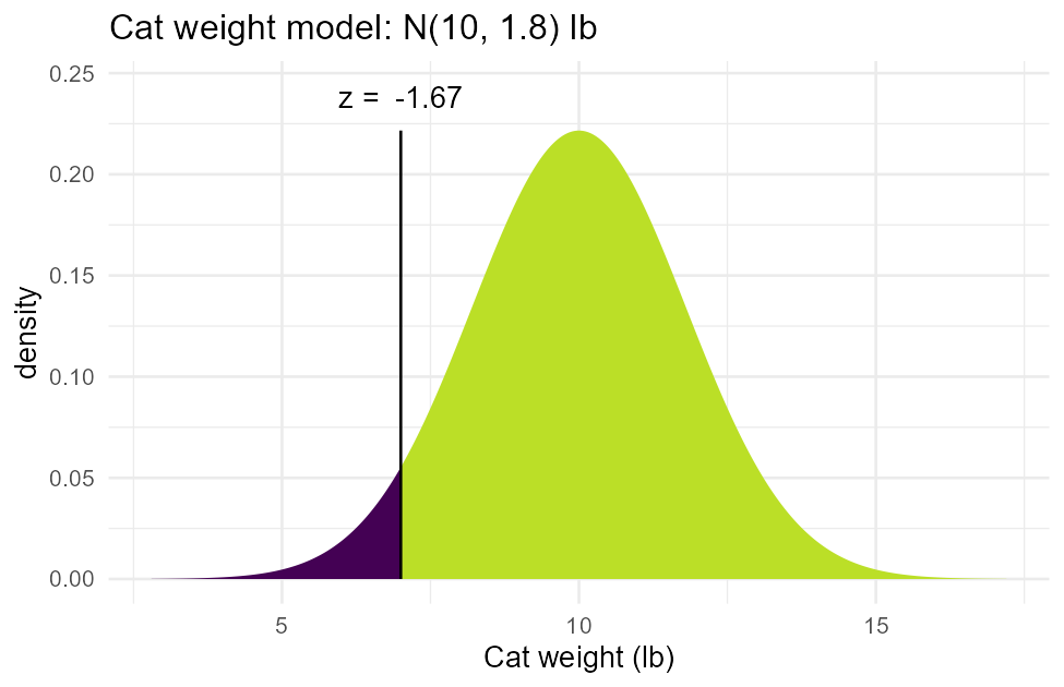
Bell curve for the cat-weight model, mean 10 lb and SD 1.8 lb, with the region below 7 lb shaded on the left tail; the shaded area covers about 4.8% of the total area under the curve.

Figure 1. A bell curve for the cat-weight model $N(10, 1.8)$ with the region below $x=7$ shaded on the left tail; the shaded area covers about 4.8% of the total area under the curve.

Bell curve for the commute-time model, mean 22 minutes and SD 6 minutes, with the region above 30 minutes shaded on the right tail; the shaded area covers about 9.1% of the total area under the curve.

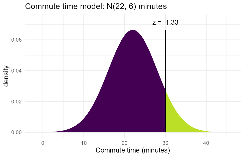
Figure 2. A bell curve for the commute-time model $N(22, 6)$ with the region above $x=30$ shaded on the right tail; the shaded area covers about 9.1% of the total area under the curve.

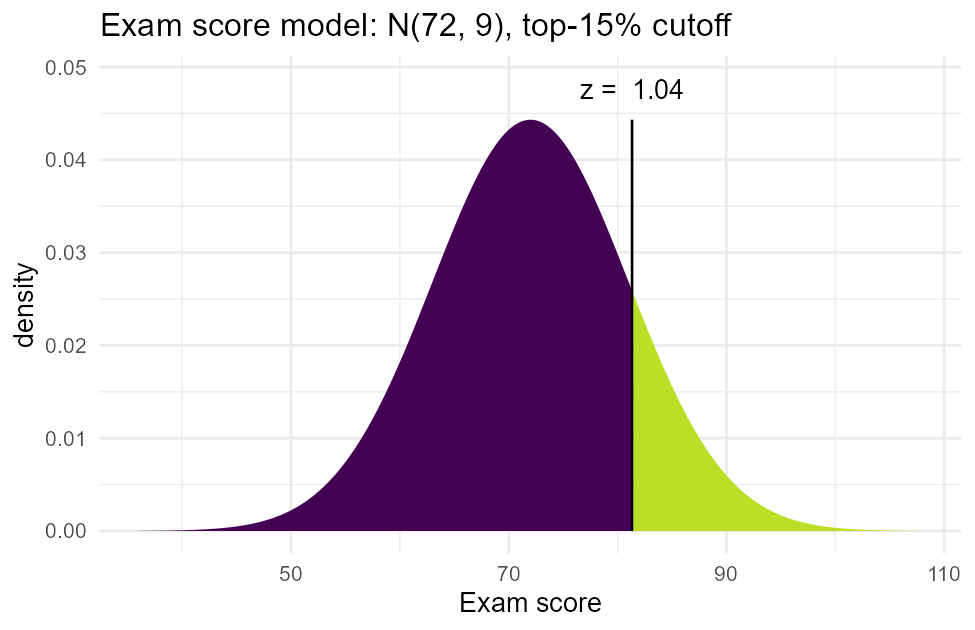
Bell curve for the exam-score model, mean 72 and SD 9, with a vertical line at 81.33; the shaded region to its right covers exactly 15% of the area, matching the target top-15% cutoff.

Figure 3. A bell curve for the exam-score model $N(72, 9)$ with a vertical line at $x=81.33$ ; the shaded region to its right covers exactly 15% of the area, matching the target top-15% cutoff.

MATH 952 skills refresher — substituting carefully, and “at least” vs. “at most”

Order of operations in $z=(x-\mu)/\sigma$ : the subtraction happens first, then you divide the whole result by $\sigma$ — treat the numerator as if it were in parentheses. For $x=7$ , $\mu=10$ , $\sigma=1.8$ : compute $7-10=-3$ first, then divide, $-3 \div 1.8 = -1.667$ . Dividing before subtracting (e.g., $7 \div 1.8$ first) gives a meaningless number.

“At least” vs. “at most”: “at least” means “this value or anything bigger” — the right tail, so you either use normalcdf(value, 1E99, μ, σ) or take the complement $1 - P(X<\text{value})$ . “At most” means “this value or anything smaller” — the left tail, read directly as normalcdf(-1E99, value, μ, σ), no complement needed. When in doubt, sketch the curve and shade the side the phrase describes before you compute anything.

4Check your understanding¶

Using the cat-weight model $N(10, 1.8)$ , a vet flags any cat under 6.5 lb as underweight. Find the z-score for 6.5 lb and the proportion of adult cats the model predicts fall below that cutoff.
In your own words, explain what a z-score of -1.11 tells you about a value relative to its population, without doing any further arithmetic.
Using the commute-time model $N(22, 6)$ , what proportion of days does the commute take at least 28 minutes? Give your z-score and state which tail of the curve you shaded.
A dean wants to model students’ Instagram-follower counts with a Normal curve. Give one reason this might be a poor fit, and name one feature of the data’s histogram you would check first.
Using the exam-score model $N(72, 9)$ , what score marks the cutoff for the top 5% of the class (a “highest honors” citation)?
Using the commute-time model $N(22, 6)$ , what proportion of days does the commute fall between 20 and 26 minutes? Write the normalcdf/xpnorm call you would use before you compute anything.

5Key terms¶

z-score — $z=(x-\mu)/\sigma$ ; how many standard deviations a value sits above (positive) or below (negative) the mean of its Normal model.
Standard Normal model, $N(0,1)$ — the Normal curve with mean 0 and SD 1 that every z-score is measured against.
z-table — a printed table of cumulative areas $P(Z<z)$ , organized by row (ones-and-tenths of $z$ ) and column (hundredths of $z$ ); stores $z$ rounded to two decimals.
normalcdf(lower, upper, μ, σ) — TI-83/84 function returning the area (probability) between two cutoffs on a Normal curve; matches xpnorm(q, mean=, sd=) in R.
invNorm(area, μ, σ) — TI-83/84 function returning the value with a given area to its left (the inverse-Normal/percentile problem); matches xqnorm(p, mean=, sd=) in R.
ShadeNorm(lower, upper, μ, σ) — TI-83/84 draw command that shades the requested region on a Normal curve.
Percentile — the value below which a stated percentage of the distribution falls (e.g., the 85th percentile has 85% of values below it).
Cutoff / threshold — the specific data value marking a probability boundary (e.g., “the score for the top 15%”).
Approximately Normal — a distribution close enough to bell-shaped and symmetric (mean near median, no long one-sided tail) that the Normal model gives trustworthy probabilities.