Week 13 — Inference for One Proportion

This week in a line: you’ll build a confidence interval and run a hypothesis test for a single population proportion.

A shelter’s adoption newsletter says “86% of our adoptions are forever homes.” A flyer outside the Student Union claims “90% of CSUB students commute rather than live on campus.” Both are claims about a population proportion — the share of an entire group that has some trait — and neither claim was checked by asking every pet owner or every student. Someone sampled a few hundred cases and reported a percentage. The last two weeks gave you the general logic of turning a sample statistic into a confidence interval and a hypothesis test: point estimate, standard error, critical value or p-value, decision. This week reuses every piece of that machinery on the single most common number in daily life — a proportion — and adds exactly one new wrinkle: a condition that tells you when the Normal-curve shortcut is trustworthy at all.

1The sample proportion and the success–failure condition¶

Let $p$ (the population proportion) be the true, usually unknown, share of a population that has some trait. You estimate it with the sample proportion,

where $x$ is the number of “successes” (cases with the trait) in a random sample of size $n$. “Success” is just labeling language borrowed from coin flips — it means “the outcome you’re counting,” not “a good outcome.” $\hat p$ is a statistic; $p$ is the parameter it estimates, exactly the population/sample distinction from Week 1.

Every method this week leans on one fact: when a sample is big enough, the sampling distribution of $\hat p$ is close to Normal, centered at $p$, with standard error $SE = \sqrt{p(1-p)/n}$ — the Week 9 idea, applied to a proportion. “Big enough” has a name, the success–failure condition: you need at least 10 expected successes and at least 10 expected failures,

(using $p_0$ in place of $\hat p$ for a hypothesis test — more on that below). You also need independence: the sample was drawn randomly, and if it was drawn without replacement from a finite population, the sample is no more than about 10% of that population. Skip the check and the whole Normal-curve shortcut — interval or test — is not trustworthy, no matter how clean the rest of the arithmetic looks.

2A confidence interval for one proportion¶

A confidence interval for $p$ takes the same shape as every interval since Week 10: point estimate ± margin of error, where the margin of error is a critical value $z^*$ times the standard error:

Note the standard error above uses $\hat p$, not $p$ — the whole point of the interval is that $p$ is unknown, so $\hat p$ is the best available stand-in. The familiar critical values return unchanged: $z^*=1.645$ for 90% confidence, $z^*=1.96$ for 95%, $z^*=2.576$ for 99%.

Worked Example 1 — are adopted pets coming back? A local animal shelter reviews its records for the past year: of $n=250$ pets adopted, $x=34$ were returned to the shelter within that first year.

Condition check. $n\hat p = 250(0.136)=34\ge10$ and $n(1-\hat p)=216\ge10$ — both comfortably clear the success–failure bar. The 250 adoption records were pulled at random from the shelter’s full adoption log and represent well under 10% of “every pet ever adopted,” so independence is reasonable too.

Building the 95% interval.

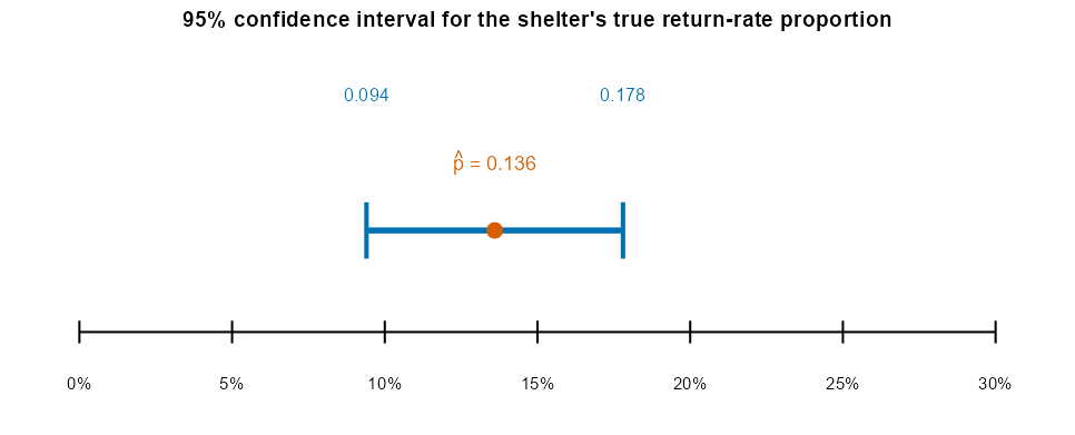
Interpretation. We are 95% confident that the true proportion of all adopted pets at this shelter that get returned within a year is between 9.4% and 17.8%. That is a statement about the method, not this one interval: if the shelter repeated this sampling process many times, about 95% of the resulting intervals would capture the true return rate. It is not correct to say “there’s a 95% probability the true rate is in this interval” — the true rate is a fixed number; it’s the interval that varies from sample to sample.

Figure 1. A number line from 0 to 0.30 marking the point estimate $\hat p=0.136$ with a dot and a horizontal bracket spanning from 0.094 to 0.178, representing the 95% confidence interval; the bracket sits entirely below 0.20, showing the true return rate is unlikely to reach 20%.

3Testing a claimed proportion: the one-proportion z-test¶

A hypothesis test starts from a specific claimed value, $p_0$, and asks whether the sample data give good evidence against it. Following Week 11’s logic exactly:

Here is the one new wrinkle: the standard error in the test statistic uses $p_0$, not $\hat p$:

Why $p_0$ and not $\hat p$? A hypothesis test is a “what if” argument: if $H_0$ were true and the population proportion really were $p_0$, how surprising would a sample proportion this far from $p_0$ be? Answering that question means describing the sampling distribution of $\hat p$ under the assumption that $p_0$ is correct — so every piece of that distribution, including its spread, is built from $p_0$. Plugging in $\hat p$ instead would quietly assume the very thing being tested. (This is also why the success–failure condition for a test checks $np_0\ge10$ and $n(1-p_0)\ge10$, not $n\hat p$.) The confidence interval has no such “what if” — there is no claimed value to test against — so it uses the only proportion it has, $\hat p$.

Once you have $z$, get the p-value the same way as any z-test: the area in the tail(s) of the standard Normal curve beyond $z$ (both tails for $\ne$, one tail for $<$ or $>$). Compare the p-value to $\alpha$ and decide.

Worked Example 2 — is the 90% commuter claim right? A campus flyer claims “90% of CSUB students commute rather than live on campus” ($p_0=0.90$). Student government surveys a random sample of $n=120$ students; $x=100$ say they commute. Test the claim at $\alpha=0.05$.

Condition check. $np_0 = 120(0.90)=108\ge10$ and $n(1-p_0)=12\ge10$ — condition holds. The sample was drawn at random, and 120 is far less than 10% of CSUB’s enrollment.

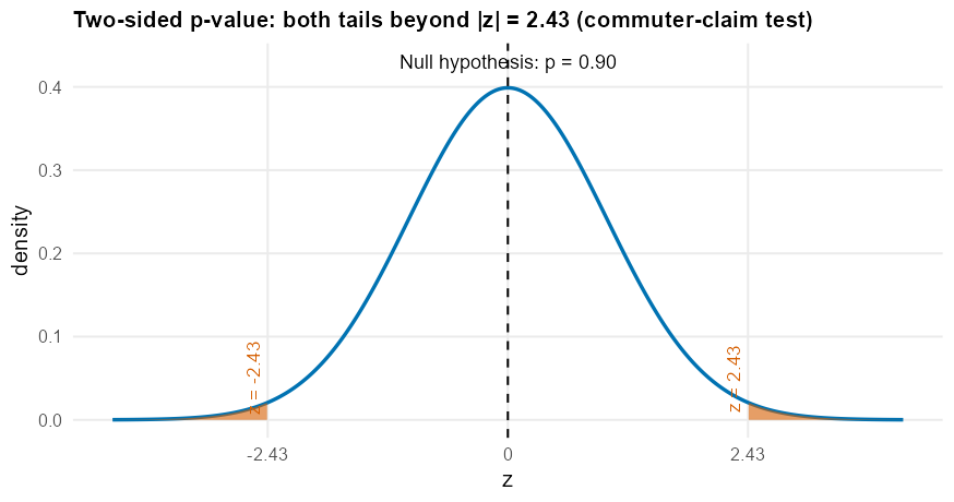
The two-sided p-value is the combined area beyond $z=\pm2.43$ under $N(0,1)$: p-value $\approx 0.0149$ (about 1.5%).

Decision. Since $0.0149 < 0.05$, we reject $H_0$. There is statistically significant evidence that the true proportion of CSUB students who commute is different from the claimed 90% — this sample’s 83.3% commuter rate is farther below 90% than we’d expect from sampling variability alone if 90% were really correct.

Figure 2. A standard Normal curve with both tails beyond $z=-2.43$ and $z=+2.43$ shaded; the two shaded slivers together represent the p-value, visibly thin compared to the whole area under the curve, matching the computed 1.49%.

See it in R.

suppressMessages({library(mosaic); library(BSDA)})

# Worked Example 1: 95% CI for the return-rate proportion
prop.test(34, 250, conf.level = 0.95)

# Worked Example 2: two-sided test of H0: p = 0.90
prop.test(100, 120, p = 0.90, alternative = "two.sided")

Running prop.test(34, 250, conf.level = 0.95) reports $\hat p = 0.136$ and a 95% interval of $(0.0973,\ 0.1863)$ — close to, but not identical to, the by-hand $(0.094,\ 0.178)$ above. prop.test(100, 120, p = 0.90, alternative = "two.sided") reports $z^2$ (as a chi-squared statistic) and p-value $=0.0225$ — close to, but not identical to, the by-hand 0.0149.

Why the small gap? By default, R’s prop.test() applies a continuity correction. It also computes a slightly different interval formula, called a “Wilson score” interval, instead of the $\hat p\pm z^*SE$ formula this course teaches by hand and on the TI-84. Adding correct = FALSE moves R’s numbers closer to the hand calculation. Either way, R agrees with the hand calculation on what matters for a decision — reject or fail to reject, and roughly where the interval sits. That agreement is the whole point of using R as a confirmation tool: it is outstanding at matching careful hand work, and a poor substitute for understanding why the numbers came out that way. Two correct methods can report slightly different decimals — recognizing that, instead of assuming one of them must be wrong, is part of learning the limits of your tools.

4Check your understanding¶

1. A coffee shop near campus claims 80% of its customers order a drink with dairy milk. A barista randomly pulls $n=80$ receipts; $x=64$ show a dairy-milk drink. Check the success–failure condition and build a 90% confidence interval for the true proportion of dairy-milk orders. Interpret it in one sentence.

2. A phone-battery maker claims 95% of its batteries last a full day of typical use without a mid-day charge. A reviewer tests $n=200$ batteries at random; $x=178$ last the full day. Test at $\alpha=0.05$ whether the true proportion differs from the claimed 95%. State $H_0$, $H_a$, and check the condition before computing anything.

3. A food-delivery app advertises that 80% of orders arrive within 30 minutes. A student group randomly samples $n=90$ delivery receipts; $x=68$ arrived within 30 minutes. Check the success–failure condition and build a 95% confidence interval for the true on-time proportion.

4. Suppose a separate campus survey of sleep habits reports a 95% confidence interval for the proportion of students who get at least 7 hours of sleep on weeknights as $(0.31,\ 0.58)$. Write one correct sentence interpreting this interval, and name one condition that had to hold for the interval to be trustworthy in the first place.

5. A streaming service claims “at least 60% of our subscribers watch primarily on a mobile device.” A sample of $n=150$ subscribers finds $x=79$ who watch primarily on mobile. Test the claim at $\alpha=0.05$ (use $H_a: p<0.60$). State $H_0$, $H_a$, check the condition, compute $z$ and the p-value, and state your conclusion in context.

6. In your own words, explain why the standard error in a one-proportion hypothesis test uses the claimed value $p_0$, while the standard error in a one-proportion confidence interval uses the sample value $\hat p$. What would go wrong if you used $\hat p$ in the test’s standard error instead?

5Key terms¶

• Population proportion, $p$ — the true share of an entire population that has some trait; a parameter, usually unknown.

• Sample proportion, $\hat p$ — $x/n$, the share of a sample with the trait; a statistic that estimates $p$.

• Success–failure condition — the check $n\hat p \ge 10$ and $n(1-\hat p)\ge10$ (or $np_0\ge10$, $n(1-p_0)\ge10$ for a test) that must hold before treating the sampling distribution of $\hat p$ as approximately Normal.

• Null proportion, $p_0$ — the specific value of $p$ claimed under $H_0$; used, not $\hat p$, inside the test’s standard error.

• One-proportion $z$-interval — $\hat p \pm z^*\sqrt{\hat p(1-\hat p)/n}$, a confidence interval for a single population proportion.

• One-proportion $z$-test — a hypothesis test of $H_0: p=p_0$ using $z=(\hat p-p_0)/\sqrt{p_0(1-p_0)/n}$.