Week 14 — Inference for One Mean - Statistics in the Modern World (MATH 1209)

This week in a line: you’ll build a confidence interval and run a hypothesis test for a single population mean, using the t-distribution.

It’s a holiday-shortened week, so campus is quieter than usual, but your two biggest new statistics tools of the semester are due right on schedule. Last week you built a confidence interval and ran a hypothesis test for a single proportion — a fraction of people who do something. This week asks the parallel question about an average instead: how long does a typical nap last between classes? Is the average commute to campus really as short as the parking office claims? Both questions need the same two moves you already know — a confidence interval, then a hypothesis test — but for a mean, those moves lean on a new reference distribution, because you almost never know the population’s true spread.

1The t-distribution: the price of not knowing $\sigma$ ¶

Back in Week 9, the standard error of a sample mean was $SE_{\bar x} = \sigma/\sqrt{n}$ , where $\sigma$ (population standard deviation) was simply given. In real problems, you almost never know $\sigma$ — all you have is your sample’s standard deviation, $s$ . Swapping in $s$ for $\sigma$ seems harmless, but it adds a second layer of guessing on top of sampling variability: $s$ itself bounces around from sample to sample, especially when $n$ is small. To account for that extra wobble, one-mean inference uses the t-distribution instead of the Normal (z) distribution whenever $\sigma$ is unknown — which is the normal state of affairs.

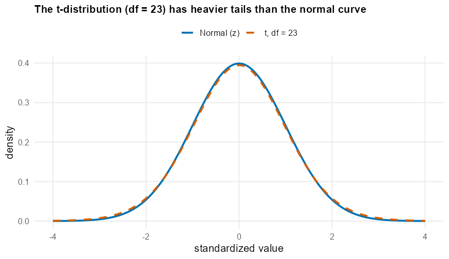
The t-distribution is bell-shaped and centered at 0, just like z, but it is flatter in the middle and has heavier tails — more area out past $\pm 2$ or $\pm 3$ — to cover the extra uncertainty from estimating $\sigma$ with $s$ . Exactly how heavy the tails are depends on the degrees of freedom, $df = n - 1$ : fewer degrees of freedom (smaller samples) means heavier tails and a wider critical value; as $n$ grows, $df$ grows, and the t-curve tightens until it is nearly indistinguishable from z. Running R’s qt() across a range of $df$ makes the convergence concrete:

$df$	5	10	20	30	50	100
$t^*$ (95% CI)	2.571	2.228	2.086	2.042	2.009	1.984

For comparison, the Normal critical value is a fixed $z^* = 1.960$ for a 95% interval. Notice how $t^*$ starts well above $z^*$ at $df = 5$ and steadily closes the gap — by $df = 100$ it is only 0.024 away from 1.960, and it would keep sliding closer as $df$ grows further. That single row of numbers is the large-sample story of this course: t and z agree closely once your sample is reasonably large, but t is the honest choice whenever $\sigma$ is estimated rather than known.

Figure 1. A t-distribution curve overlaid on a standard Normal curve, both centered at 0 and bell-shaped, shows the t-curve sitting slightly lower at the peak and slightly higher than the Normal curve out past $\pm 2$ on both sides — the “heavier tails” that make $t^*$ larger than $z^*$ for the same confidence level.

A t-distribution curve (df = 23) overlaid on a standard Normal curve, both centered at 0 and bell-shaped. The t-curve sits slightly lower at the peak and slightly higher than the Normal curve out past plus-or-minus 2 on both sides, showing the heavier tails that make t-star larger than z-star for the same confidence level.

2A confidence interval for a mean¶

Conditions first. Before building an interval, check: (1) independence — observations come from a random sample or a random process, so one value doesn’t influence another; (2) large sample or nearly normal — with $n \geq 30$ the Central Limit Theorem covers you even if the data are somewhat skewed; with smaller $n$ , the sample should show no strong skew and no extreme outliers.

With those conditions met, the confidence interval for a population mean $\mu$ is

\bar{x} \pm t^* \cdot \frac{s}{\sqrt{n}}

where $\bar{x}$ is the sample mean, $s$ is the sample standard deviation, $n$ is the sample size, $s/\sqrt{n}$ is the standard error of the mean, and $t^*$ is the critical value cut from the t-distribution with $df = n-1$ degrees of freedom at the chosen confidence level.

Worked Example 1 — how long is a CSUB short nap?

A random sample of $n = 24$ students who nap between classes reported their most recent nap length in minutes (nap_minutes_sim, a seeded simulation):

20,\ 51,\ 18,\ 38,\ 35,\ 9,\ 28,\ 34,\ 10,\ 22,\ 19,\ 35,\ 10,\ 24,\ 9,\ 57,\ 21,\ 32,\ 23,\ 18,\ 32,\ 21,\ 26,\ 20

Conditions. The sample is random, so observations are reasonably independent. favstats() gives $Q_1 = 18.75$ and $Q_3 = 32.5$ , so $IQR = 13.75$ and the upper outlier fence is $32.5 + 1.5(13.75) = 53.125$ ; the 57-minute nap is a mild outlier, and 51 is not. With $n = 24$ and only one mild outlier (no extreme skew), the near-normal condition is reasonably satisfied for a teaching example, though a stricter analysis would flag the 57 for a closer look.

Summary statistics: $\bar{x} = 25.5$ minutes, $s = 12.24$ minutes, $n = 24$ .

Standard error: $SE_{\bar x} = s/\sqrt{n} = 12.24/\sqrt{24} = 2.50$ minutes.

Critical value: $df = n - 1 = 23$ ; for 95% confidence, $t^* = 2.069$ (from the t-table row for $df = 23$ ).

Margin of error: $ME = t^* \cdot SE_{\bar x} = 2.069 \times 2.50 = 5.17$ minutes.

Interval: $25.5 \pm 5.17 = (20.33,\ 30.67)$ minutes.

Interpretation: we are 95% confident that the true mean nap length among CSUB students who nap between classes is between about 20.3 and 30.7 minutes. This is a statement about the method’s long-run reliability, not a probability about this one interval.

Figure 2. A number line from 15 to 35 minutes marking the sample mean $\bar x=25.5$ with a dot and a horizontal bracket spanning from 20.33 to 30.67, representing the 95% confidence interval for the true mean nap length.

A number line from 15 to 35 minutes marking the sample mean x-bar equals 25.5 with a dot and a horizontal bracket spanning from 20.33 to 30.67, the 95 percent confidence interval for the true mean nap length.

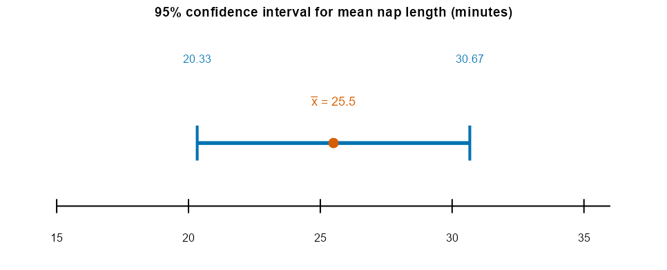
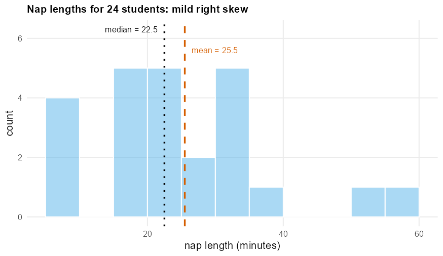
Figure 3. A histogram of the 24 nap lengths is mounded between about 10 and 35 minutes with a thin tail stretching out to 51 and 57 minutes — a mild right skew, consistent with the mean (25.5 minutes) sitting a bit above the median (22.5 minutes) and with the single flagged outlier at 57.

A histogram of the 24 nap lengths, mounded between about 10 and 35 minutes with a thin tail stretching out to 51 and 57 minutes, a mild right skew. A dashed line marks the mean at 25.5 minutes and a dotted line marks the median at 22.5 minutes, with the single flagged outlier visible at 57.

3The one-sample t-test for a mean¶

A hypothesis test for a mean checks a claim about $\mu$ using the same ingredients. The null hypothesis states a specific value, $H_0: \mu = \mu_0$ ; the alternative $H_a$ says $\mu$ differs from $\mu_0$ (two-sided) or is specifically greater than or less than it (one-sided). The test statistic is

t = \frac{\bar{x} - \mu_0}{s/\sqrt{n}}, \qquad df = n - 1,

and the p-value is the area under the t-curve with $df = n-1$ degrees of freedom, out past the observed $t$ in the direction(s) $H_a$ points. As always: small p-value (below your significance level $\alpha$ ) means the data are surprising under $H_0$ , so you reject $H_0$ ; otherwise you fail to reject $H_0$ .

Worked Example 2 — is the campus commute really only 20 minutes?

CSUB’s parking and transportation office advertises an average commute of 20 minutes for commuter students. A random sample of $n = 45$ commuter students (commute_min_sim) reports $\bar{x} = 23.49$ minutes and $s = 9.39$ minutes. Many students suspect the true average is longer than advertised, so this calls for a one-sided test.

Hypotheses: $H_0: \mu = 20$ minutes vs. $H_a: \mu > 20$ minutes.

Conditions. The sample is random, and $n = 45 \geq 30$ , so the large-sample condition covers any mild skew in commute times.

Standard error: $SE_{\bar x} = 9.39/\sqrt{45} = 1.40$ minutes.

Test statistic: $df = 44$ ,

t = \frac{23.49 - 20}{1.40} = 2.49.

p-value: the area under the $t_{44}$ curve above $t = 2.49$ is $p = 0.0083$ .

Decision: at $\alpha = 0.05$ , $p = 0.0083 < 0.05$ , so we reject $H_0$ .

Conclusion in context: the sample gives strong evidence that the true mean commute time for CSUB commuter students exceeds the advertised 20 minutes.

Large samples: why t and z nearly agree. Re-running Example 2’s exact summary statistics through the z-based equivalent (same $\bar x$ , $s$ , and $n$ , but referenced against the Normal curve instead of $t_{44}$ ) gives $z = 2.49$ — the identical test statistic value, because the formula is the same — with $p = 0.0064$ , versus the t-test’s $p = 0.0083$ . The two p-values are close enough that both lead to the same decision at $\alpha = 0.05$ , exactly the pattern the $t^*$ -vs- $z^*$ table above predicted: once $n$ is large (here $df = 44$ ), the extra uncertainty from estimating $\sigma$ with $s$ barely matters, and t and z tell the same story. For small samples, they can disagree more, which is why this course leads with t.

See it in R.

suppressMessages({library(mosaic); library(BSDA)})

# Worked Example 1: nap length, confidence interval from raw data
nap_minutes_sim <- c(20, 51, 18, 38, 35, 9, 28, 34, 10, 22, 19, 35,
                      10, 24, 9, 57, 21, 32, 23, 18, 32, 21, 26, 20)
naps <- data.frame(nap_minutes_sim)
favstats(~ nap_minutes_sim, data = naps)
t.test(~ nap_minutes_sim, data = naps, conf.level = 0.95)$conf.int

# Worked Example 2: commute time, one-sample t-test from summary stats (BSDA)
tsum.test(mean.x = 23.49, s.x = 9.39, n.x = 45, mu = 20, alternative = "greater")

# large-sample z equivalent, same summary stats (noted, not required)
zsum.test(mean.x = 23.49, sigma.x = 9.39, n.x = 45, mu = 20, alternative = "greater")

t.test()$conf.int returns 20.33286 30.66714, matching Example 1’s hand-built interval. tsum.test() returns t = 2.4933, df = 44, p-value = 0.008246, matching Example 2. zsum.test() on the identical summary numbers returns z = 2.4933, p-value = 0.006329 — the same test statistic, a slightly smaller p-value, and the same decision at $\alpha = 0.05$ , exactly the t-vs-z agreement described above. Use tsum.test()/zsum.test() whenever a problem only gives you $\bar{x}$ , $s$ (or $\sigma$ ), and $n$ rather than a raw data list.

MATH 952 skills refresher — dividing by a square root, and reading a t-table row

Standard error is a two-step calculation. $SE_{\bar x} = s/\sqrt{n}$ means: (1) take the square root of $n$ first, (2) then divide $s$ by that result — never divide first. For Example 1: $\sqrt{24} \approx 4.899$ , then $12.24 / 4.899 \approx 2.50$ . Skipping straight to “ $12.24/24$ ” gives a wrong, much smaller number.

Reading a t-table. A printed t-table has one row per $df$ and one column per confidence level (or per tail area). Find your row ( $df = n-1$ ), then the column for your confidence level, and read off $t^*$ — no interpolation needed for the values used in this course. The row for $df = 23$ (Example 1) reads:

$df$	90%	95%	99%
23	1.714	2.069	2.807

Notice $t^*$ grows as confidence grows (a wider interval to be more sure) — the same pattern you saw with $z^*$ back in Week 10.

4Check your understanding¶

A campus wellness survey plans to estimate mean daily screen time from a random sample of $n = 18$ students. The sample’s histogram shows one clear peak, roughly symmetric shape, and no outliers. Is it reasonable to use t-procedures here? Explain using both conditions from this week (independence, and sample size/shape).
A sample of $n = 36$ receipts at a campus café gives $\bar{x} = \$6.40$ and $s = \$1.80$ . Find the standard error of the mean. (Do not build the full interval yet — just the standard error.)
A sample of $n = 16$ phone battery-life tests gives $\bar{x} = 8.2$ hours and $s = 1.6$ hours. Construct and interpret a 90% confidence interval for the true mean battery life.
Using the t-table row for $df = 23$ from this week’s skills refresher, what is $t^*$ for a 99% confidence interval? How does it compare to the 95% value used in Worked Example 1, and why does a higher confidence level need a larger $t^*$ ?
A streaming service claims subscribers watch an average of 90 minutes per day. A random sample of $n = 20$ subscribers gives $\bar{x} = 97$ minutes and $s = 15$ minutes. Test $H_0: \mu = 90$ vs. $H_a: \mu > 90$ at $\alpha = 0.05$ , showing the test statistic, $df$ , p-value, decision, and a one-sentence conclusion in context.
Explain, in your own words, why $t^*$ is larger than $z^*$ for the same confidence level when $n$ is small, and why that gap shrinks as $n$ grows. Use the $df$ -vs- $t^*$ table from this week to support your answer.

5Key terms¶

Standard error of the mean ( $SE_{\bar x}$ ) — $s/\sqrt{n}$ ; how much sample means typically vary from the true population mean.
t-distribution — a bell-shaped distribution like the Normal curve, but with heavier tails, used for mean inference when the population SD $\sigma$ is unknown (estimated by $s$ ).
Degrees of freedom ( $df$ ) — for one-mean inference, $df = n - 1$ ; controls how heavy the t-distribution’s tails are.
Critical value ( $t^*$ ) — the t-value cutting off the confidence level’s tail area(s); larger than the matching $z^*$ for small $df$ , converging to it as $df$ grows.
Confidence interval for a mean — $\bar{x} \pm t^* \cdot s/\sqrt{n}$ .
One-sample t-test — tests $H_0: \mu = \mu_0$ using $t = (\bar{x} - \mu_0)/(s/\sqrt{n})$ with $df = n-1$ .
TInterval / T-Test — the TI-83/84 menu items (under STAT ▸ TESTS) for a one-mean confidence interval and hypothesis test.
t.test() / tsum.test() / zsum.test() — the matching R functions: t.test() from raw data (mosaic), tsum.test() from summary statistics, and zsum.test() as the large-sample z equivalent when $\sigma$ is treated as known (BSDA).