Week 15 — Review (Ch 6–7) & Course Wrap-up - Statistics in the Modern World (MATH 1209)

This week in a line: no new material — this is your Chapters 6–7 review, the comprehensive final-exam study guide, and the course wrap-up.

Fifteen weeks ago you met a claim — “coffee drinkers live longer,” “the shelter’s most playful cats get adopted fastest” — and learned to ask how do they know that? before you believed it. Since then you’ve built, one week at a time, an entire toolkit for answering that question with data instead of guessing. You classified variables and studies (Ch 1), learned to summarize a batch of numbers or categories honestly (Ch 2), reasoned about chance with probability and expected value (Ch 3), met the Normal curve and learned to compute exact areas and percentiles under it (Ch 4), and then spent the second half of the semester on the two ideas that connect the whole course: a confidence interval estimates an unknown population value, and a hypothesis test checks whether a specific claimed value is believable, once you account for ordinary sampling variability (Ch 5). The last two chapters put that logic to work on the two most common real-world questions — what percent...? (Ch 6, one proportion) and what’s the average...? (Ch 7, one mean). This week does three things: it finishes reinforcing Chapter 7 (last week’s holiday-shortened session moved fast, so this is your second look before Quiz 7), it gives you a Chapters 6–7 review checklist, and it hands you a complete study plan for the comprehensive final. There is no new content this week — every idea below is one you have already met.

1The arc of the semester, in seven steps¶

If you can say what each line below means and give one example of your own, you have the whole course in your hands:

Data & study design (Ch 1) — where the numbers came from, and whether the design supports a cause-and-effect claim.
Summarizing data (Ch 2) — turning a messy list of numbers or categories into a handful of trustworthy numbers and honest graphs.
Probability (Ch 3, §3.1) — the rules for combining chances (complement, addition, multiplication) and what “independent” means.
Random variables & the Normal curve (Ch 3, §3.4–3.5 → Ch 4) — expected value and spread of a chance process, and exact areas/percentiles under a bell curve.
Sampling distributions, CIs, and testing logic (Ch 5) — why a sample statistic wobbles from sample to sample, and the two general tools (interval, test) built on that fact.
Inference for one proportion (Ch 6) — the tools of step 5, made concrete for a percentage question.
Inference for one mean (Ch 7) — the same tools, made concrete for an average question.

Every later step uses the machinery of the steps before it — nothing in this course is a free-standing fact you memorized in isolation. That’s also why the final is comprehensive: a one-mean test (step 7) only makes sense if you still remember what a p-value is (step 5) and why standard deviation matters (step 2).

2Review checklist: Chapter 6 — Inference for One Proportion (Week 13)¶

Recognize a one-proportion scenario: the variable of interest is categorical with two outcomes (success/failure), and the question is about the population proportion $p$ having that outcome.
Check the success–failure condition before trusting the Normal-based procedure: for a test, $n p_0 \ge 10$ and $n(1-p_0) \ge 10$ using the claimed proportion $p_0$ ; for an interval, $n\hat p \ge 10$ and $n(1-\hat p)\ge 10$ using the sample proportion $\hat p$ . Also check the sample is random/independent.
Build a confidence interval: $\hat p \pm z^* \cdot SE_{\hat p}$ , where $SE_{\hat p} = \sqrt{\hat p (1-\hat p)/n}$ — the standard error uses $\hat p$ (you don’t know $p$ ; you’re trying to estimate it).
Run a hypothesis test: state $H_0: p = p_0$ vs. $H_A: p \ne p_0$ (or $<, >$ for a one-sided claim); the test statistic $z = (\hat p - p_0)/SE_{p_0}$ uses $SE_{p_0} = \sqrt{p_0(1-p_0)/n}$ — this time the standard error uses the claimed value $p_0$ , because the test asks “if $p_0$ were true, how surprising is my $\hat p$ ?”
State the decision (reject / fail to reject $H_0$ ) by comparing the p-value to $\alpha$ , then translate that decision into a plain-language conclusion about the original claim, not just about $H_0$ .

3Review checklist: Chapter 7 — Inference for One Mean (Week 14–15)¶

Recognize a one-mean scenario: the variable of interest is numerical, and the question is about the population mean $\mu$ .
Check conditions: the sample is random/independent, and the sample is either large ( $n \ge 30$ is the usual rough guideline) or shows no strong skew/outliers if smaller — you cannot skip this check just because $n$ “feels big enough.”
Build a confidence interval: $\bar x \pm t^* \cdot SE_{\bar x}$ , where $SE_{\bar x} = s/\sqrt{n}$ and $t^*$ comes from the t-distribution with $df = n-1$ degrees of freedom (not the same $z^*$ you used in Ch 6, though the two are close for large $n$ ).
Run a hypothesis test: state $H_0: \mu = \mu_0$ vs. $H_A$ ; the test statistic is $t = (\bar x - \mu_0)/(s/\sqrt n)$ , again with $df = n-1$ .
Remember the reason we lead with t rather than z here: your text and your TI-84’s native menu (TInterval/T-Test) both use $t$ , and $t$ automatically becomes almost identical to $z$ once $n$ is large — you are not learning two different ideas, just one idea with a slightly more honest standard curve for finite samples.
As in Ch 6: translate the reject/fail-to-reject decision into a sentence about the original claim, in the original units (hours, dollars, minutes — never just “ $\mu$ ”).

On your TI-83/84 & in R — the cross-procedure drill

Practice reaching for the right menu item / function without being told the chapter — that’s exactly what the final will ask you to do.

Task	TI-83/84	R (`mosaic`/`BSDA`)
Normal area (probability)	`2ND VARS(DISTR) ▸ normalcdf(lower,upper,μ,σ)`	`xpnorm(q, mean=, sd=)`
Normal percentile (inverse)	`invNorm(area,μ,σ)`	`xqnorm(p, mean=, sd=)`
One-proportion interval	`STAT ▸ TESTS ▸ 1-PropZInt`	`prop.test(x, n, conf.level=)$conf.int`
One-proportion test	`STAT ▸ TESTS ▸ 1-PropZTest`	`prop.test(x, n, p=, alternative=, correct=FALSE)`
One-mean interval	`STAT ▸ TESTS ▸ TInterval`	`tsum.test(mean.x=, s.x=, n.x=, conf.level=)$conf.int`
One-mean test	`STAT ▸ TESTS ▸ T-Test`	`tsum.test(mean.x=, s.x=, n.x=, mu=)`

(In R, correct = FALSE tells prop.test() to skip the continuity correction it applies by default, so its p-value matches the TI-84’s 1-PropZTest and the by-hand formula you learned — worth remembering if you ever compare the two and the p-values look slightly different.)

4The comprehensive final: a Chapter 1–7 checklist¶

The final is cumulative — every chapter you’ve studied gets at least one question, plus at least one item that asks you to choose the right procedure with no chapter label attached. Work through this list chapter by chapter; if a bullet feels shaky, that chapter’s weekly unit has the full worked example.

4.1Chapter 1 — Data & Study Design¶

Variable types (numerical: discrete/continuous; categorical: nominal/ordinal) · population vs. sample, parameter vs. statistic · sampling methods and sources of bias · observational study vs. experiment, and why only randomization supports a cause-and-effect claim (confounding). (The full worked version of this checklist is in Week 7’s review.)

4.2Chapter 2 — Summarizing Data¶

Mean, median, mode, standard deviation $s$ , five-number summary, IQR, the 1.5·IQR outlier rule · shape (symmetric / skewed / modality) and why skew pulls the mean away from the median · frequency/relative-frequency tables and honest (zero-based) bar charts · two-way tables and the difference between a marginal, joint, and conditional proportion. (Full worked version also in Week 7’s review.)

4.3Chapter 3 — Probability, Random Variables & the Normal Curve¶

Sample space and probability as long-run relative frequency · complement rule $P(A^c)=1-P(A)$ · addition rule (general and disjoint) · multiplication rule for independent events · a discrete random variable’s distribution (probabilities sum to 1) · expected value $E(X)=\sum x P(x)$ · $SD(X)=\sqrt{\sum (x-\mu)^2 P(x)}$ · continuous variables: probability = area under a density curve · features of the Normal curve · z-scores $z=(x-\mu)/\sigma$ · the 68–95–99.7 empirical rule.

4.4Chapter 4 — Working with the Normal Model¶

Finding an exact proportion below/above/between given values (normalcdf/xpnorm) · finding the value at a given percentile (invNorm/xqnorm) · judging whether the Normal model is even appropriate for a given variable (and saying so when it isn’t — that’s a graded skill, not an afterthought).

4.5Chapter 5 — Sampling Distributions, Confidence Intervals & Testing Logic¶

Point estimate ( $\hat p$ , $\bar x$ ) vs. population parameter ( $p$ , $\mu$ ) · why a statistic varies from sample to sample (sampling variability) · standard error, $SE_{\hat p}=\sqrt{p(1-p)/n}$ and $SE_{\bar x}=s/\sqrt n$ · the Central Limit Theorem, in plain words · a confidence interval’s correct interpretation (a range of plausible values for the parameter at a stated confidence level — not “there’s a 95% probability the parameter is in this particular interval”) · $H_0$ / $H_A$ , p-value, $\alpha$ , and the reject/fail-to-reject decision · Type I error (rejecting a true $H_0$ ) vs. Type II error (failing to reject a false $H_0$ ), and the real-world cost of each · statistical significance vs. practical importance.

4.6Chapter 6 — Inference for One Proportion¶

See the checklist above — success–failure condition, $\hat p \pm z^*SE_{\hat p}$ for an interval, $z=(\hat p - p_0)/SE_{p_0}$ for a test.

4.7Chapter 7 — Inference for One Mean¶

See the checklist above — large/near-normal-sample condition, $\bar x \pm t^* (s/\sqrt n)$ for an interval, $t=(\bar x - \mu_0)/(s/\sqrt n)$ , $df=n-1$ , for a test.

5Which procedure do I use? A decision guide¶

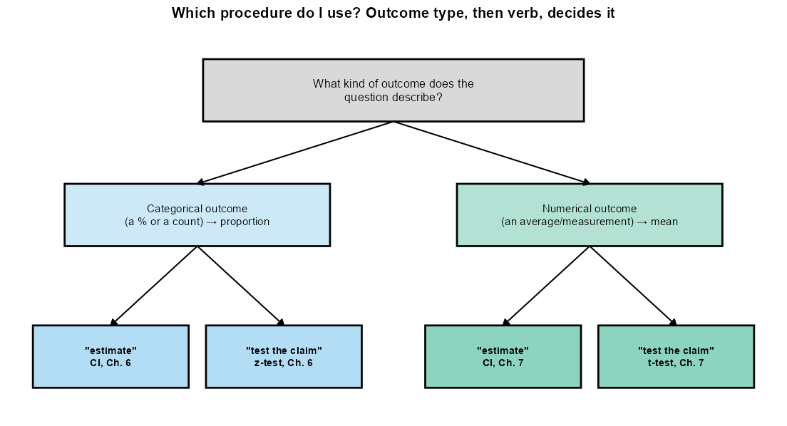
This course only ever studies one group at a time — you will never be asked to compare two proportions or two means (that’s Ch 6.2–7.5, outside this course). That simplifies the final’s “which tool?” question to a short chain:

Figure 1. A two-stage decision-flow diagram: first the outcome type (categorical vs. numerical) sets proportion vs. mean, then the verb (estimate vs. test the claim) sets confidence interval vs. hypothesis test.

A two-stage decision-flow diagram. A top box asks, what kind of outcome does the question describe? Two arrows lead to categorical outcome, a percent or a count, which points to proportion; and numerical outcome, an average or measurement, which points to mean. Each of those splits again into estimate, leading to a confidence interval, and test the claim, leading to a hypothesis test, giving four leaves: proportion CI (Chapter 6), proportion z-test (Chapter 6), mean CI (Chapter 7), and mean t-test (Chapter 7).

Is the question about how the data were collected, or about a cause-and-effect claim? → Chapter 1 vocabulary (population/sample, observational study/experiment, confounding). No calculation needed.
Does the question just ask you to describe or graph a dataset — no unknown population value is being estimated? → Chapter 2 (numerical or categorical summary).
Does the question hand you probabilities directly, or a full probability distribution, and ask you to combine them or find an expected value? → Chapter 3 (probability rules, $E(X)$ , $SD(X)$ ).
Does the question say a variable “is approximately Normal” and ask for an area or a percentile — with no sample statistic being used to estimate an unknown parameter? → Chapter 4 (normalcdf/invNorm, xpnorm/xqnorm).
Is the question about the standard error, the sampling distribution itself, or testing vocabulary (Type I/II error, what a p-value measures) rather than a full computed answer? → Chapter 5.
Does the question give you a sample proportion or count (a “percent who...” / “yes-or-no” outcome) and ask you to estimate or test a population proportion? → Chapter 6. Categorical outcome → proportion.
Does the question give you a sample mean (an “average...” / a numerical measurement) and ask you to estimate or test a population mean? → Chapter 7. Numerical outcome → mean.

Once you’re in step 6 or 7, one more fork decides interval vs. test — watch the verb:

If the question says...	You need a...
“estimate,” “construct a range for,” “how confident can we be,” “what interval...”	Confidence interval
“test the claim,” “is there evidence that,” “has changed,” “differs from,” “is greater/less than a stated value,” “at the $\alpha=\dots$ level”	Hypothesis test

Final exam logistics

Coverage: comprehensive, Chapters 1–7. By teaching-time weighting: Data/summaries (Ch 1–2) ≈ 20%, Probability/Normal (Ch 3–4) ≈ 20%, Inference foundations (Ch 5) ≈ 25%, One proportion (Ch 6) ≈ 17%, One mean (Ch 7) ≈ 18%. Every chapter gets at least one item, plus at least one item that tests your ability to choose the right procedure.
Length: the standard 105-minute final period (confirm your exact room/time block against the Registrar’s finals-week grid, Dec 9–15); about 34 items total, mixing at most ~6 multiple-choice questions (≤ 18% of the exam) with short-answer and free-response problems where you must show your work.
Closed book, closed notes. You may bring two handwritten 8.5″×11″ formula sheets, front and back (formulas/notation only, no worked examples) — both are collected with your exam.
Calculator: TI-83/84 (or your instructor’s stated equivalent). No phone calculators.
No makeup finals, and remember the standing policy: if you missed Exam 1, Exam 2 already counted double for you; if you missed Exam 2, this final now absorbs its 20% weight on top of the final’s own 25% — treat your preparation accordingly if either applies to you.
Exams are printed in 5 equivalent randomized forms (A–E); content and difficulty are the same across forms.

6Mixed exam-style worked examples¶

Cover each solution with a sheet of paper, work the problem yourself, then check your steps. Every number below was computed in R (mosaic/BSDA, R 4.5.2, set.seed(1209)), so you can trust it to the decimal place.

Example 1 (Ch 1) — Design and vocabulary at the shelter

The animal shelter from Week 1’s opening wants to know whether a short “meet & greet” session (15 minutes with a potential adopter, before any adoption decision) increases the chance that a cat is adopted within two weeks. Staff randomly assign 30 of this month’s 60 new cats to get a meet & greet and the other 30 to the usual process; two weeks later, each cat is marked adopted or not.

Explanatory variable: meet & greet vs. usual process — categorical, nominal (two unordered labels).
Response variable: adopted within two weeks (yes/no) — categorical, nominal.
Observational study or experiment? Experiment — staff themselves assigned the treatment (which cats got the meet & greet), rather than observing an existing pattern.
Does this design support a cause-and-effect claim? Yes — because the 60 cats were randomly split into the two groups, the groups should be similar, on average, in every other trait that might affect adoption (breed, age, temperament, coat color). If the meet & greet group is adopted at a noticeably higher rate, a confounding variable can’t easily explain it away, so the difference is attributable to the meet & greet itself. A shelter that instead just compared cats whose current foster families happened to arrange informal meet & greets against those that didn’t could not rule out confounding this cleanly — maybe more sociable cats already get informal meet & greets and get adopted faster, for the same underlying reason (their temperament), not because of the meet & greet.

Example 2 (Ch 2) — Numerical and categorical summaries at the coffee shop

Part A — numerical. During Monday’s morning rush, the coffee shop times 10 customers’ wait, in minutes, from order to pickup: 3, 4, 3.5, 5, 4, 3, 4.5, 3, 4, 12 (the last customer waited through a card-reader glitch).

suppressMessages({library(mosaic); library(BSDA)})
wait <- c(3, 4, 3.5, 5, 4, 3, 4.5, 3, 4, 12)
favstats(wait)
#>  min    Q1 median    Q3 max mean       sd  n missing
#>    3 3.125      4 4.375  12  4.6 2.685351 10       0

Five-number summary: min = 3, $Q_1=3.125$ , median = 4, $Q_3=4.375$ , max = 12. $IQR = 4.375-3.125 = 1.25$ , so the outlier fences are $Q_1-1.5(IQR)=1.25$ and $Q_3+1.5(IQR)=6.25$ . The 12-minute wait sits well above 6.25 — a formally flagged outlier — which is exactly why the mean (4.6 min) sits noticeably above the median (4 min): one slow transaction pulled the mean upward, but the median barely moved. Report the median (or the mean with the outlier noted) as the fairer “typical” wait.

Part B — categorical. The same shop cross-tabulates 200 customers’ ordering method (App vs. Counter) against drink temperature (Hot vs. Iced):

coffee <- matrix(c(40, 70, 60, 30), nrow = 2,
                  dimnames = list(Drink = c("Hot", "Iced"),
                                   Method = c("App", "Counter")))
coffee
#>       Method
#> Drink  App Counter
#>   Hot   40      60
#>   Iced  70      30
prop.table(coffee, margin = 2)   # conditional on each column (method)
#>       Method
#> Drink        App   Counter
#>   Hot  0.3636364 0.6666667
#>   Iced 0.6363636 0.3333333

Marginal: overall, $100/200 = 0.500$ , so 50.0% of all 200 orders were iced, ignoring method.
Joint: $70/200 = 0.350$ , so 35.0% of all 200 customers both ordered by app and got an iced drink.
Conditional: among app orders, $70/110 = 0.636$ (63.6% iced); among counter orders, $60/90 = 0.667$ , so only $30/90=0.333$ (33.3%) ordered iced.

Read-back: the conditional iced rate swings from 63.6% (app) to 33.3% (counter) — a 30-point gap — so ordering method and drink temperature appear associated. That makes sense: app orders are placed ahead for pickup (more time to want a cold specialty drink), while early counter walk-ins during a chilly morning rush lean hot.

Example 3 (Ch 3) — Probability rules and a tip-jar random variable

Part A — probability rules. Among this month’s shelter intakes, 55% are cats ( $P(\text{cat})=0.55$ ) and 30% are adopted within one week ( $P(\text{adopted}\le 1wk)=0.30$ ). Assume, for this exercise, that species and one-week adoption are independent.

pCat <- 0.55; pAdopt <- 0.30
p_and <- pCat * pAdopt
p_or  <- pCat + pAdopt - p_and
c(p_and = p_and, p_or = p_or, `1-pAdopt` = 1 - pAdopt)
#>     p_and      p_or 1-pAdopt
#>     0.165     0.685     0.700

Multiplication rule (independence): $P(\text{cat and adopted}\le 1wk) = 0.55(0.30)=0.165$ — 16.5% of intakes are cats adopted within a week. Addition rule: $P(\text{cat or adopted}\le1wk) = 0.55+0.30-0.165 = 0.685$ — 68.5% are one or the other (or both). Complement: $P(\text{not adopted}\le1wk) = 1-0.30 = 0.70$ — 70% are still unadopted a week in.

Part B — expected value. The shop’s tip jar receives $0, $1, $2, or $5 tips with probabilities 0.50, 0.30, 0.15, 0.05.

tip <- c(0, 1, 2, 5); p <- c(0.50, 0.30, 0.15, 0.05)
sum(p)                                  # check it's a valid distribution
#> [1] 1
mu <- sum(tip * p); mu
#> [1] 0.85
sqrt(sum((tip - mu)^2 * p))
#> [1] 1.19478

The distribution is valid ( $0.50+0.30+0.15+0.05=1$ ). $E(\text{tip}) = 0(.50)+1(.30)+2(.15)+ 5(.05) = \$0.85$ — the average tip per customer, in the long run. $SD(\text{tip}) \approx \$1.19$ tells you individual tips vary quite a bit around that $0.85 average (most tip $0 or $1, but a few $5 tips pull the spread up).

Example 4 (Ch 3.5 / Ch 4) — Normal model: phone battery life

Suppose (as a model for this exercise) a phone’s battery life is approximately Normal with $\mu=11$ hours and $\sigma=1.5$ hours. What’s the chance a battery lasts more than 14 hours, and what battery life marks the top 10% of phones?

z <- (14 - 11) / 1.5
z
#> [1] 2
xpnorm(14, mean = 11, sd = 1.5)
#> If X ~ N(11, 1.5), then
#>   P(X <= 14) = P(Z <= 2) = 0.9772
#>   P(X >  14) = P(Z >  2) = 0.02275
xqnorm(0.90, mean = 11, sd = 1.5)
#> If X ~ N(11, 1.5), then
#>   P(X <= 12.92233) = 0.9
#>   P(X >  12.92233) = 0.1

Standardizing gives $z = (14-11)/1.5 = 2.0$ , so a 14-hour battery is exactly 2 standard deviations above the mean. The exact Normal calculation says only about 2.275% of batteries last longer than 14 hours — close to the empirical rule’s “about 2.5% beyond 2 SDs,” confirming the rule was a good approximation, not a coincidence. The battery life at the 90th percentile — the cutoff for the longest-lasting 10% of phones — is about 12.92 hours (found by “inverse Normal”: working backward from an area to a value, exactly what invNorm/xqnorm are built for).

Example 5 (Ch 5) — Testing logic: the campus rec-fee poll, revisited

Back in Week 9, two reporters each polled 50 students about a proposed recreation-fee increase and got 52% and 50% support — different numbers from ordinary sampling variability. Suppose the paper later runs one larger, fresh random sample of $n=200$ students and finds $x=112$ in favor. Administration’s official position is that support is exactly 50% ( $p_0 = 0.50$ ); the paper wants to test whether support is actually above 50%.

$H_0: p = 0.50$ vs. $H_A: p > 0.50$ (one-sided, since the paper’s suspicion has a direction).

Conditions: $np_0 = 200(0.50)=100$ and $n(1-p_0)=100$ — both comfortably $\ge 10$ , and the sample is random, so the Normal-based test applies.

n <- 200; x <- 112; p0 <- 0.50
phat <- x / n
SE0 <- sqrt(p0 * (1 - p0) / n)
z <- (phat - p0) / SE0
pval <- 1 - pnorm(z)
c(phat = phat, SE0 = SE0, z = z, pval = pval)
#>      phat       SE0         z      pval
#> 0.5600000 0.0353553 1.6970563 0.0448430

$\hat p = 112/200 = 0.560$ . The standard error, using the claimed value $p_0=0.50$ (this is a test, not an interval), is $SE_{p_0}=\sqrt{0.5(0.5)/200}=0.0354$ . The test statistic is $z=(0.560-0.500)/0.0354 = 1.70$ , giving a one-sided p-value of 0.0448.

Decision: $0.0448 < \alpha = 0.05$ , so we reject $H_0$ — the critical value for a one-sided $\alpha=0.05$ test is $z^*=1.645$ (qnorm(0.95)), and our $z=1.70$ clears it. There is statistically significant evidence, at the 5% level, that support for the fee increase exceeds 50%.

A worthwhile wrinkle. The (informational, two-sided) 95% confidence interval for $p$ here works out to about $(0.491,\ 0.629)$ — and notice it still contains 0.50. That isn’t a contradiction: a one-sided test at $\alpha=0.05$ and a two-sided 95% interval answer subtly different questions, and this example sits right at the boundary between them. It’s a good reminder that “statistically significant” can be a close call, and that significance is not the same as a large, decisive gap — exactly the Ch 5 distinction between statistical and practical importance.

Example 6 (Ch 6 + Ch 7) — The hardest combined example: one proportion, one mean

Part A — one proportion. The shelter claims 65% of animals are adopted within 30 days. In a review of the last 150 intakes, 87 were adopted within 30 days. Test, at $\alpha=0.05$ , whether the true 30-day adoption rate differs from the claimed 65%, and give a 95% confidence interval for the true rate.

$\hat p = 87/150 = 0.580$ . Conditions for the test: $np_0=150(0.65)=97.5$ , $n(1-p_0)=52.5$ — both $\ge 10$ . $H_0: p=0.65$ vs. $H_A: p \ne 0.65$ (two-sided, since we’re just checking the claim, with no direction suspected).

n <- 150; x <- 87; phat <- x/n; p0 <- 0.65
SE0 <- sqrt(p0*(1-p0)/n)
z   <- (phat - p0)/SE0
pval <- 2*(1 - pnorm(abs(z)))
c(phat = phat, z = z, pval = pval)
#>       phat          z       pval
#>  0.5800000 -1.7974341  0.0722667

SEhat <- sqrt(phat*(1-phat)/n)
ME <- qnorm(0.975)*SEhat
c(lower = phat - ME, upper = phat + ME)
#>     lower     upper
#> 0.5010156 0.6589844

Test statistic $z=(0.580-0.650)/\sqrt{0.65(0.35)/150} = -1.80$ , two-sided p-value $=0.0723$ . Since $0.0723 > 0.05$ , we fail to reject $H_0$ — this sample does not give strong enough evidence, at the 5% level, that the true 30-day adoption rate differs from 65%. The 95% confidence interval, $\hat p \pm z^*\sqrt{\hat p(1-\hat p)/n} = 0.580 \pm 1.96(0.0403) \approx (0.501,\ 0.659)$ , is consistent with that decision: it comfortably contains 0.65.

Part B — one mean. A wellness survey during finals week samples $n=28$ CSUB students’ nightly sleep and finds $\bar x = 6.4$ hours, $s=1.3$ hours. The commonly recommended amount of adult sleep is 8 hours. Test, at $\alpha=0.05$ , whether mean finals-week sleep differs from 8 hours, and give a 95% confidence interval.

$H_0: \mu=8$ vs. $H_A: \mu \ne 8$ . Conditions: the sample is random/independent, and with $n=28$ and no reported extreme skew or outliers, the t-procedure is appropriate.

tsum.test(mean.x = 6.4, s.x = 1.3, n.x = 28, mu = 8,
          alternative = "two.sided", conf.level = 0.95)
#>  One-sample t-Test
#> data:  Summarized x
#> t = -6.5126, df = 27, p-value = 5.546e-07
#> 95 percent confidence interval:
#>  5.895913 6.904087
#> sample estimates:
#> mean of x
#>       6.4

$t=(6.4-8)/(1.3/\sqrt{28}) = -6.51$ on $df=27$ , with p-value $\approx 0.0000006$ — far below $\alpha=0.05$ . We reject $H_0$ : there is very strong evidence that mean sleep during finals week differs from (and is below) 8 hours. The 95% CI, about $(5.90,\ 6.90)$ hours, sits entirely below 8, which is exactly why the test rejected so decisively — the interval and the test are telling you the same story from two angles.

Which-test check: Part A’s outcome (“adopted within 30 days?”) is categorical → a proportion procedure (Ch 6, prop.test-style). Part B’s outcome (hours of sleep) is numerical → a mean procedure (Ch 7, tsum.test). If you can see that split instantly on the final, you’ve mastered this week’s real objective.

7What belongs on your two formula sheets¶

Your two 8.5″×11″ sheets (front and back each) may hold formulas, symbols, and short notes — no worked examples. Handwriting this table yourself, rather than printing it, is real review: it forces you to notice which formulas you already have memorized.

Concept	Formula	Symbols
Sample mean / SD	$\bar x=\dfrac{\sum x_i}{n}$ , $\;s=\sqrt{\dfrac{\sum(x_i-\bar x)^2}{n-1}}$	$n$ = sample size
IQR / outlier fences	$IQR=Q_3-Q_1$ ; fences $Q_1-1.5\,IQR$ , $Q_3+1.5\,IQR$	$Q_1,Q_3$ = quartiles
Complement / addition / multiplication	$P(A^c)=1-P(A)$ ; $P(A\text{ or }B)=P(A)+P(B)-P(A\text{ and }B)$ ; $P(A\text{ and }B)=P(A)P(B)$ if independent	—
Expected value / SD of a r.v.	$E(X)=\sum xP(x)$ ; $SD(X)=\sqrt{\sum(x-\mu)^2P(x)}$	$\mu=E(X)$
z-score / empirical rule	$z=\dfrac{x-\mu}{\sigma}$ ; 68–95–99.7 within 1/2/3 $\sigma$	$\mu,\sigma$ = population mean, SD
Standard errors	$SE_{\hat p}=\sqrt{\dfrac{p(1-p)}{n}}$ ; $SE_{\bar x}=\dfrac{s}{\sqrt n}$	—
General CI	point estimate ± (critical value) $\times SE$	—
One-proportion CI / test	$\hat p \pm z^*SE_{\hat p}$ (SE uses $\hat p$ ); $z=\dfrac{\hat p - p_0}{\sqrt{p_0(1-p_0)/n}}$ (SE uses $p_0$ )	$p_0$ = claimed proportion
One-mean CI / test	$\bar x \pm t^*\dfrac{s}{\sqrt n}$ ; $t=\dfrac{\bar x-\mu_0}{s/\sqrt n}$ , $df=n-1$	$\mu_0$ = claimed mean

Symbol legend (memorize; don’t waste sheet space): $\mu$ vs. $\bar x$ ; $\sigma$ vs. $s$ ; $p$ vs. $\hat p$ ; $n$ ; $H_0$ / $H_A$ ; $\alpha$ ; $p_0$ / $\mu_0$ (the claimed value under a test).

Final-exam day tips

Budget time by chapter weight: on a 105-minute final, that’s roughly 21 minutes on Ch 1–2 material, 21 minutes on Ch 3–4, 26 minutes on Ch 5, 18 minutes on Ch 6, and 19 minutes on Ch 7. Don’t let one stubborn early question eat the time you need for Ch 5’s logic questions, which carry the most weight.
Before any inference problem, write the condition check ( $np_0\ge10$ / large-or-near-normal sample) — even a quick line earns partial credit and catches setup errors early.
State $H_0$ / $H_A$ in symbols and in words before you compute anything; a right answer to the wrong hypotheses earns little credit.
Watch the verb: “estimate/construct a range” → interval; “test the claim/is there evidence” → hypothesis test. Watch the direction word too: “differs from” is two-sided; “more than,” “less than,” “has increased/decreased” is one-sided.
Sketch and shade a Normal (or t) curve for every inference problem, even when not required — it catches sign errors before you commit to a final answer.
Say “reject $H_0$ ” or “fail to reject $H_0$ ” — never “accept $H_0$ .” A test that fails to reject never proves the null is true, only that this sample didn’t give strong enough evidence against it.
Bring your TI-83/84 with fresh batteries and both handwritten formula sheets. No phones.
If you finish early, revisit every inference conclusion and check it’s written in context (about adoption rates or sleep hours — not just “ $p$ ” or “ $\mu$ ”).

8Check your understanding¶

Brief answers follow so you can self-check; no full step-by-step solutions are given here on purpose — if yours doesn’t match, redo the matching worked example above before the final.

In Example 1, if the shelter instead just compared cats whose foster families happened to arrange their own informal meet & greets against those that didn’t, what kind of study would that be, and why would it weaken the cause-and-effect claim? (Observational; a confounding variable like the cat’s own temperament could explain both the informal meet & greet and the faster adoption.)
In Example 2’s coffee-wait data, which single value, if removed, would pull the mean closest to the median — and why does the median barely move when you remove it? (The 12-minute outlier; the median depends only on the middle-ranked values, so one extreme value at either end has almost no effect on it.)
Is “35.0% of all 200 customers ordered by app and got an iced drink” (Example 2) a marginal, joint, or conditional proportion? (Joint.)
In Example 3, if species and one-week adoption were not independent, could you still use $P(\text{cat})\times P(\text{adopted}\le1wk)$ to find $P(\text{cat and adopted}\le1wk)$ ? (No — the multiplication rule in that simple form requires independence; without it you’d need the actual joint probability from data.)
In Example 4, would a battery life of 9.5 hours correspond to a positive or a negative z-score, and roughly how many SDs from the mean is it? (Negative; $z=(9.5-11)/1.5 \approx -1$ , about 1 SD below the mean.)
In Example 5, if the paper’s new sample had instead found $x=105$ out of $n=200$ (52.5%), would you expect the p-value to be larger or smaller than 0.0448? Why, without recomputing? ( $\hat p$ closer to $p_0=0.50$ means a smaller gap to explain away, so the p-value would be larger — less evidence against $H_0$ .)
In Example 6 Part A, is “the true 30-day adoption rate” a parameter or a statistic? Is 0.580 a parameter or a statistic? (The true rate is the parameter $p$ , unknown; 0.580 is the sample statistic $\hat p$ .)
A campus survey question reads: “Estimate the average number of hours per week CSUB students spend on campus.” Interval or test — and proportion or mean? (Confidence interval, because the word is “estimate”; mean, because “average...hours” is a numerical outcome — this is a Chapter 7 confidence-interval question.)

9Key terms¶

success–failure condition — the check ( $np\ge10$ and $n(1-p)\ge10$ ) that justifies using a Normal-based procedure for a proportion.
null proportion $p_0$ / null mean $\mu_0$ — the specific claimed value being tested against the sample data in $H_0$ .
one-proportion z-interval / z-test — the Ch 6 procedures for estimating or testing a single population proportion $p$ .
standard error of the mean, $SE_{\bar x}=s/\sqrt n$ — how much a sample mean typically varies from sample to sample.
t-distribution — the slightly wider, bell-shaped curve used for one-mean inference, indexed by its degrees of freedom.
degrees of freedom, $df=n-1$ — the parameter that determines the exact shape of the t-distribution for a one-sample t-procedure.
T-interval / T-test — the Ch 7 procedures for estimating or testing a single population mean $\mu$ .
which-test decision language — the habit of reading a scenario for its variable type (categorical/numerical) and its verb (estimate/test) before choosing a procedure.

10A closing note¶

You started this course being asked to trust — or doubt — a claim about coffee, sleep, or shelter cats. You now have a reason for every doubt and a method for every trust: a study design to critique, a graph to build honestly, a probability rule to apply, a Normal curve to shade, a standard error to compute, and — for the two most common real questions a workplace or a newsroom ever asks, what percent...? and what’s the average...? — a confidence interval and a hypothesis test you can build and defend from scratch. That is not a small thing. Whatever you do after this semester — nursing, business, criminal justice, education, something you haven’t decided yet — you will meet a percentage, an average, or a claim dressed up as a fact, and you will be one of the people in the room who knows how to ask whether it holds up. Good luck on the final. You’ve already done the hard part.