Random Variables and the Normal Model

library(mosaic)
library(BSDA)
library(ggplot2)
knitr::opts_chunk$set(
  message = FALSE, warning = FALSE,
  fig.align = "center", fig.width = 7, fig.height = 4.2,
  dpi = 150, out.width = "85%"
)
# Okabe-Ito colorblind-safe palette used throughout this chapter
# (defined inline; 1 blue, 2 orange, 3 bluishgreen, 4 vermillion, ...).
ok <- c("#0072B2", "#E69F00", "#009E73", "#CC79A7",
        "#56B4E9", "#D55E00", "#F0E442", "#999999")
blue   <- ok[1]   # "#0072B2"
orange <- ok[2]   # "#E69F00"
green  <- ok[3]   # "#009E73"

1A Kern hook: how tall is a Bakersfield adult?¶

Stand at the entrance to a CSUB lecture hall and watch people walk in. Most are clustered around a typical height; a few are noticeably short, a few noticeably tall, and the farther you get from “typical,” the rarer the person. If you tallied everyone’s height and drew the picture, you would get a single hump, roughly symmetric, thinning out on both sides — the famous bell curve.

We do not have to imagine it. The nhanes_subset dataset is a real teaching sample of body measurements from the U.S. CDC’s National Health and Nutrition Examination Survey (the codebook calls it a teaching sample, not a survey-weighted population estimate — we use it to learn methods, not to make official claims about U.S. adults). Let us look at the standing height of the adult men in it.

nh <- read.csv("data/processed/nhanes_subset.csv")
men <- subset(nh, sex == "male" & age >= 20 & !is.na(height_cm))
c(n = nrow(men),
  mean_cm = round(mean(men$height_cm), 2),
  sd_cm   = round(sd(men$height_cm), 2))

There are 3,524 adult men in the sample, with a mean height of 175.79 cm (about 5 ft 9 in) and a standard deviation of 7.48 cm (dataset-derived from nhanes_subset; see the codebook in data/codebooks/nhanes_subset.md). Here is the picture, with a bell curve laid on top:

mu_m <- mean(men$height_cm)
sd_m <- sd(men$height_cm)

ggplot(men, aes(x = height_cm)) +
  geom_histogram(aes(y = after_stat(density)), bins = 30,
                 fill = blue, colour = "white") +
  stat_function(fun = dnorm, args = list(mean = mu_m, sd = sd_m),
                colour = "black", linewidth = 1) +
  labs(x = "Height (cm)", y = "Density",
       title = "Adult male height with a Normal model overlaid") +
  theme_minimal(base_size = 12)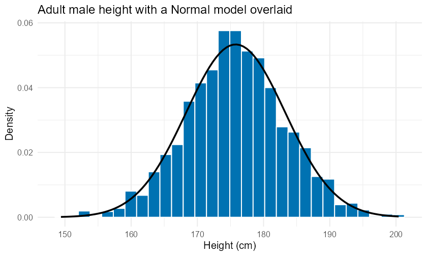

Histogram of standing height for 3,524 adult men in the NHANES teaching sample, with a Normal(175.79 cm, 7.48 cm) curve overlaid. The data form a single symmetric hump that the bell curve tracks closely.

This chapter is about that curve and the machinery behind it. We will first make precise what a random variable is and how to find its average and spread. Then we will study the most important continuous model in all of statistics — the Normal model — and learn to read probabilities and percentiles off of it. Finally we will meet the binomial model for counting successes, and we will practice the most important skill of all: deciding whether a Normal model is even appropriate before you trust it.

2Learning objectives¶

By the end of this chapter you will be able to:

1. Define a random variable and compute the expected value and variance of a discrete random variable.

2. State the properties of the Normal distribution and the 68–95–99.7 rule.

3. Standardize values to z-scores and find Normal probabilities and percentiles using xpnorm / xqnorm (the mosaic teaching versions of base R’s pnorm / qnorm).

4. Use the binomial model for counts of successes and identify when it applies.

5. Assess whether the Normal model is appropriate for a given variable using a histogram and 68–95–99.7 reasoning.

31. Random variables¶

3.1Intuition¶

A random variable is just a number whose value depends on the outcome of a random process. Before you flip three coins you do not know how many heads you will get — it could be 0, 1, 2, or 3 — so “the number of heads” is a random variable. Before you draw a random Bakersfield summer day you do not know its PM2.5 level, so “the PM2.5 level of a random day” is a random variable.

A discrete random variable can only take separated values you could in principle list (0, 1, 2, 3 heads). A continuous random variable can take any value in an interval (a height could be 175.79 or 175.794 or anything between). This chapter handles both: discrete first (counting), then continuous (the Normal model).

Two questions describe a random variable: what value do we get on average? and how much does it bounce around? Those are the expected value and the variance.

3.2Formula¶

A discrete random variable $X$ is described by its probability distribution: a list of the values $x_i$ it can take and the probability $P(X = x_i)$ of each. The probabilities are between 0 and 1 and add to 1.

The expected value (or mean) of $X$, written $E(X)$ or $\mu$ (Greek “mu,” the population mean), is the probability-weighted average of its values:

where

• $x_i$ = each value the variable can take,

• $P(X = x_i)$ = the probability of that value,

• $\sum_i$ = “add up over all the values.”

The variance of $X$, written $\operatorname{Var}(X)$ or $\sigma^2$ (Greek “sigma squared”), measures spread as the expected squared distance from the mean:

These two forms are not two different formulas — they are the same expression written two ways (expand the square $(x_i-\mu)^2$ and simplify, and the first collapses into the second). Use whichever is easier; the second form, $E(X^2) - \mu^2$, is usually quicker by hand because you only sum the squared values once. The standard deviation is $\sigma = \sqrt{\sigma^2}$, back in the original units.

3.3R¶

R has no special object for a discrete distribution — you just store the values and probabilities as two vectors and use weighted sums. Here is the whole toolkit:

# Values and their probabilities (must sum to 1).
x <- c(0, 1, 2, 3)
p <- c(0.40, 0.35, 0.20, 0.05)
sum(p)                      # check: probabilities add to 1

mu  <- sum(x * p)           # expected value  E(X) = sum x_i p_i
EX2 <- sum(x^2 * p)         # E(X^2)
var <- EX2 - mu^2           # variance = E(X^2) - mu^2
sd  <- sqrt(var)            # standard deviation

round(c(mean = mu, variance = var, sd = sd), 4)

This prints $E(X) = 0.9$, $\operatorname{Var}(X) = 0.79$, and $\sigma = 0.8888$. We work through where these come from in Section 7.1.

42. The Normal model¶

4.1Intuition¶

Many measurements pile up in the same shape: one central hump, symmetric, thinning toward both tails. Adult height does it. Measurement errors do it. Averages of many small effects do it (you will see why in Chapter 6). When a variable has that shape, we can describe its entire distribution with just two numbers — its center and its spread — using the Normal model.

The Normal model is a smooth curve, not a set of bars, because the variable is continuous. The area under the curve over an interval is the probability of landing in that interval, and the total area is 1. Tall part of the curve = common values; thin tails = rare values.

The single most useful fact about the Normal model is the 68–95–99.7 rule (the “empirical rule”): about 68% of the data fall within 1 standard deviation of the mean, about 95% within 2, and about 99.7% within 3. That rule turns “mean and SD” into a full mental picture.

4.2Formula¶

We write

to mean “$X$ follows a Normal model with mean $\mu$ and standard deviation $\sigma$.” (Some books write $N(\mu, \sigma^2)$ with the variance; this book always uses the standard deviation $\sigma$ in the second slot — watch for that when you read other sources.)

To compare a value to the model we standardize it into a z-score:

where

• $x$ = the value you observed,

• $\mu$ = the mean of the model,

• $\sigma$ = the standard deviation of the model,

• $z$ = the number of standard deviations $x$ sits above ($z>0$) or below ($z<0$) the mean.

A z-score erases the units: $z = 1.5$ means “1.5 SDs above the mean” whether $x$ is a height in cm or a test score in points. The standard Normal, $N(0, 1)$, is the Normal model of z-scores themselves.

Every “what fraction is below this value?” question follows the same three-step road map, and it is worth naming the steps before you see them in code:

1. Standardize. Turn the raw value $x$ into a z-score with $z = (x-\mu)/\sigma$ — this is why we standardize: it moves any Normal question onto the single standard $N(0,1)$ scale, so one table (or one function) handles them all.

2. Look up the area. Find the fraction of the standard Normal that lies to the left of $z$. That fraction is the probability $P(X \le x)$.

3. Adjust for the question asked. For “greater than,” subtract from 1; for “between two values,” subtract the two left-areas. (Step 3 is just bookkeeping about which piece of the curve you want.)

In R, pnorm(x, mean = mu, sd = sigma) quietly does steps 1 and 2 in one call, which is why you rarely compute the z-score by hand once you trust the tool — but knowing the steps is what lets you catch a wrong answer.

Two functions answer the two questions you will ever ask of a Normal model:

• Probability (area): given a cutoff, what fraction of the curve is to one side? In R this is pnorm(x, mean = mu, sd = sigma) = $P(X \le x)$.

• Quantile (percentile): given a fraction $p$, what value cuts off that much area on the left? In R this is qnorm(p, mean = mu, sd = sigma) = the value $x$ with $P(X \le x) = p$.

These are inverses of each other.

4.3R¶

The mosaic package gives us xpnorm() and xqnorm() — teaching versions of base R’s pnorm/qnorm that show their work. Each one prints the z-score and the tail areas and draws the Normal curve with the region shaded, so you see the picture behind the number. Start by using xpnorm() to confirm the 68–95–99.7 rule on this specific model: what share of adult men fall within 1 SD of the mean?

# Show the 68-95-99.7 rule on the adult-male height model: the share within 1 SD.
# xpnorm shades the band from one SD below the mean to one SD above it.
xpnorm(c(mu_m - sd_m, mu_m + sd_m), mean = mu_m, sd = sd_m)

xpnorm prints the area to the left of each edge of the band — about 0.159 below $\mu - \sigma$ and 0.841 below $\mu + \sigma$ — and shades the two regions on the curve. The middle band is their difference, $0.841 - 0.159 = \textbf{0.6827}$: the 68% the empirical rule promises. Now use xpnorm() for a tail area and xqnorm() for a percentile:

# What fraction of adult men are taller than 180 cm?  P(X >= 180)
xpnorm(180, mean = mu_m, sd = sd_m, lower.tail = FALSE)

Here xpnorm reports the z-score ($z = 0.56$) and shades the upper tail: the printed P(X > 180) = 0.287 says about 29% of adult men clear 180 cm.

# How tall is the 90th-percentile man?  (the value with 90% of area to its left)
xqnorm(0.90, mean = mu_m, sd = sd_m)

Going the other direction, xqnorm shades the lower 90% and prints the cutoff: the 90th-percentile man is about 185.4 cm tall.

The plain base-R equivalents — which these teaching versions wrap — are 1 - pnorm(180, mu_m, sd_m) and qnorm(0.90, mu_m, sd_m). They return the same numbers, just without the printed z-score or the shaded picture. Use whichever you like.

53. The binomial model¶

5.1Intuition¶

Some random variables are counts of successes: how many of 10 random adult men are taller than 180 cm, how many of 20 patients respond to a drug, how many of 8 free throws go in. When each trial is a yes/no with the same success probability, the trials are independent, and the number of trials is fixed, the count follows the binomial model.

You should reach for the binomial only when all four conditions hold (a handy mnemonic is BINS):

• Binary — each trial is success/failure,

• Independent — trials do not influence each other,

• Number of trials $n$ is fixed in advance,

• Same success probability $p$ on every trial.

5.2Formula¶

If $X$ counts the successes in $n$ independent trials each with success probability $p$, then $X$ follows a binomial model, written $X \sim \text{Binomial}(n, p)$, and

where

• $n$ = the number of trials,

• $p$ = the success probability on each trial,

• $k$ = the particular count of successes you are asking about (an integer from 0 to $n$),

• $\binom{n}{k} = \dfrac{n!}{k!\,(n-k)!}$ = the number of ways to choose which $k$ of the $n$ trials are the successes. Here $n!$ (read “$n$ factorial”) means multiply $n$ all the way down to 1 — for example $5! = 5\cdot4\cdot3\cdot2\cdot1 = 120$.

Its mean and standard deviation have tidy closed forms:

5.3R¶

Base R provides the binomial directly: dbinom(k, n, p) for $P(X = k)$ and pbinom(k, n, p) for $P(X \le k)$.

# In the NHANES adult-male sample, the share taller than 180 cm is:
p180 <- mean(men$height_cm > 180)
round(p180, 4)

# Treat that share as p ~ 0.27. In a random group of n = 10 adult men,
# how likely is it that exactly 3 are over 180 cm?
dbinom(3, size = 10, prob = 0.27)

# And the mean and SD of the count out of 10:
n <- 10; p <- 0.27
c(mean = n * p, sd = sqrt(n * p * (1 - p)))

The observed share over 180 cm is 0.2730 in nhanes_subset (dataset-derived); rounding to $p = 0.27$ for a clean teaching number, a group of 10 has expected count $np = 2.7$ over 180 cm.

64. Is the Normal model appropriate?¶

6.1Intuition¶

The Normal model is powerful, but it is a choice, and the wrong choice gives confident wrong answers. The model is appropriate when the data are unimodal (one hump), roughly symmetric, and free of strong outliers. It is the wrong choice for skewed data, for counts bounded at zero that pile up near the bound, or for distributions with two humps.

The fastest check is a histogram: does it look like one symmetric bell? A second check is the empirical rule: compute the share of data actually within 1 and 2 SDs of the mean and compare to 68% and 95%.

6.2R¶

Adult male height passed both checks (the histogram in ch05-fig-hook is a clean bell). Now look at a variable where the Normal model fails: daily PM2.5 in Kern County (kern_airquality), which the codebook flags as right-skewed with winter inversion spikes.

air <- read.csv("data/processed/kern_airquality.csv")
pm <- subset(air, pollutant == "PM2.5")

ggplot(pm, aes(x = daily_mean)) +
  geom_histogram(bins = 40, fill = orange, colour = "white") +
  labs(x = "Daily mean PM2.5 (micrograms / cubic meter)", y = "Count of monitor-days",
       title = "Kern PM2.5: a right-skewed distribution (Normal model fails)") +
  theme_minimal(base_size = 12)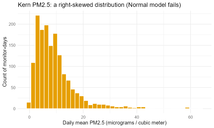

Daily PM2.5 means at Kern County monitors in 2023 (1,554 monitor-days). The distribution is strongly right-skewed — a long tail of high-pollution winter days — so a Normal model does not fit.

# Empirical-rule check: for a good Normal fit, about 68% of values lie within 1 SD.
m <- mean(~ daily_mean, data = pm)
s <- sd(~ daily_mean, data = pm)
c(mean       = round(m, 2),
  median     = round(median(~ daily_mean, data = pm), 2),
  within_1sd = round(mean(pm$daily_mean > m - s & pm$daily_mean < m + s), 3))

The mean PM2.5 is 9.30 µg/m³ but the median is only 7.56 (both dataset-derived from kern_airquality; see data/codebooks/kern_airquality.md, which reports mean PM2.5 = 9.2956). Mean far above median is the fingerprint of a right skew — and the empirical-rule check agrees: 83.7% of days fall within one SD of the mean, well above the 68% a Normal model predicts. A Normal model would predict negative pollution days (impossible) and would badly underestimate the high-pollution tail. Do not fit a bell to this.

7Worked examples¶

7.1Example 1 — Expected value and variance of a discrete random variable¶

Air-quality forecasters classify a weekend day as “good,” “moderate,” or “unhealthy.” Over a long record, a random Bakersfield summer weekend day is unhealthy with probability 0.05, moderate with 0.20, otherwise good. Let $X$ = the number of unhealthy-or-moderate days in a fixed weekend with the value assignments below. Its distribution (a teaching distribution, chosen for clean arithmetic) is:

Intuition. Most weekends have 0 or 1 such day; 3 is rare. So the average should sit below 1, and the spread should be modest.

Formula. $\mu = \sum x_i P(X=x_i)$ and $\sigma^2 = E(X^2) - \mu^2$.

Computation.

x <- c(0, 1, 2, 3); p <- c(0.40, 0.35, 0.20, 0.05)
mu  <- sum(x * p)
var <- sum(x^2 * p) - mu^2
round(c(mean = mu, variance = var, sd = sqrt(var)), 4)

Interpretation. On average 0.9 such days per weekend, give or take about 0.89 days. The mean is below 1, as our intuition predicted, and you cannot actually observe “0.9 days” — the expected value is a long-run average, not a guaranteed outcome.

7.2Example 2 — A z-score on Kern-relevant data¶

A CSUB student is 190 cm tall (about 6 ft 3 in). Using the adult-male Normal model from the NHANES teaching sample, $N(175.79, 7.48)$, how unusual is that?

Intuition. 190 is well above the mean of about 176, so we expect a solidly positive z-score, somewhere near 2.

Formula. $z = (x - \mu)/\sigma$.

Computation.

xpnorm(190, mean = mu_m, sd = sd_m)

Read the z-score straight off the printout: xpnorm reports P(Z <= 1.9), so the z-score is 1.90, and it shades everything below 190 cm on the curve. By hand: $z = (190 - 175.79)/7.48 = 1.90$.

Interpretation. This student is 1.90 standard deviations above the mean adult-male height. By the empirical rule, only about 2.5% of values lie more than 2 SDs above the mean, so a 190 cm man is in roughly the top few percent — tall, but not extraordinarily so.

7.3Example 3 — Normal probability between two values¶

Still using $N(175.79, 7.48)$ for adult-male height, what fraction of men are between 170 and 185 cm?

Intuition. That range straddles the mean and is a bit wider than $\pm 1$ SD on each side, so we expect well over half — maybe two-thirds.

Formula. $P(170 \le X \le 185) = P(X \le 185) - P(X \le 170)$, each found by standardizing and using pnorm.

Computation.

# P(170 <= X <= 185) = P(X <= 185) - P(X <= 170).
# xpnorm shades and prints the area left of each cutoff; diff() subtracts them.
diff(xpnorm(c(170, 185), mean = mu_m, sd = sd_m))

xpnorm shades both cutoffs and prints the area to the left of each — about 0.219 below 170 cm and 0.891 below 185 cm — and diff() subtracts them to give the area between.

Interpretation. About 0.6715, i.e. roughly 67% of adult men fall between 170 and 185 cm under this model. As a check, the actual share in the data is:

mean(men$height_cm > 170 & men$height_cm < 185)

0.6737 — the model’s 0.6715 matches the data’s 0.6737 to within a fraction of a percent (both dataset-derived from nhanes_subset), which is exactly why we trust the Normal model here.

7.4Example 4 — A binomial count¶

About 27% of adult men in the sample are taller than 180 cm. In a randomly chosen pickup basketball lineup of 5 adult men, what is the probability that at least 2 are over 180 cm? Give the expected number too.

Intuition. Each man independently has a 0.27 chance of clearing 180 cm, the count is out of $n=5$, so this is binomial with $n=5$, $p=0.27$. The expected count is $5 \times 0.27 \approx 1.35$, so “at least 2” should be a bit less than even odds.

Formula. $P(X \ge 2) = 1 - P(X = 0) - P(X = 1)$ with $P(X=k) = \binom{n}{k} p^k (1-p)^{n-k}$; mean $= np$.

Computation.

n <- 5; p <- 0.27
p_at_least_2 <- 1 - pbinom(1, size = n, prob = p)   # 1 - P(X <= 1)
round(p_at_least_2, 4)
n * p                                                # expected count

Interpretation. There is about a 41% chance that at least 2 of the 5 are over 180 cm, and on average 1.35 of the 5 will be. The conditions hold well enough for a teaching example — each man is roughly independent and shares the same population rate — though a real lineup of friends might violate independence (tall people cluster in basketball).

7.5Example 5 — Judging model fit (Kern dataset)¶

Should you describe Kern County daily PM2.5 (kern_airquality) with a Normal model?

Intuition. Pollution can spike enormously on bad winter days but cannot go below zero, so we expect a right skew — and a skew kills the Normal model.

Formula / tool. Compare mean vs. median, and run the empirical-rule check by hand: compute the observed share of values within $\pm 1$ SD and $\pm 2$ SD of the mean. If the within-1-SD share is far from 68% (or the within-2-SD share far from 95%), the model is suspect.

Computation.

pm_vals <- subset(read.csv("data/processed/kern_airquality.csv"),
                  pollutant == "PM2.5")$daily_mean
round(c(mean = mean(pm_vals), median = median(pm_vals)), 4)

# Empirical-rule check: for a Normal fit these shares should be near 0.68 and 0.95.
m <- mean(pm_vals); s <- sd(pm_vals)
round(c(within_1sd = mean(pm_vals > m - s   & pm_vals < m + s),
        within_2sd = mean(pm_vals > m - 2*s & pm_vals < m + 2*s)), 4)

Interpretation. The mean (9.30) sits well above the median (7.56) — the signature of right skew — and the histogram (ch05-fig-fit-fail) confirms one long upper tail. The empirical-rule check makes the misfit concrete: 83.7% of days fall within 1 SD of the mean (a Normal predicts 68%); the skew crowds too many quiet days near the mean and strands a few extreme days far out in the tail. The Normal model is not appropriate here; describe this variable with the median and IQR (Chapter 2) instead, and never quote “68% within one SD” for it.

8Try it¶

• Shiny — Statistics Explorer, “Sampling Distribution” module. Choose a population shape (including a Normal population you set with $\mu$ and $\sigma$) or a Binomial$(n,p)$ proportion, and watch the simulated distribution form; every button shows the exact mosaic R code it ran, so you can paste it back here. Launch with shiny::runApp("shiny-explorer") from the repo root.

• Jupyter lab: labs/lab05-random-variables-normal.ipynb walks you through computing $E(X)$ and $\operatorname{Var}(X)$ by hand, reading pnorm/qnorm, and running your own empirical-rule fit check on a dataset of your choice.

Looking ahead — the t-distribution and the Normal. The standard Normal $N(0,1)$ you just learned has a close cousin, the Student’s $t$-distribution, that you will lean on for inference in later chapters. It looks almost like the Normal but with heavier tails when information is scarce, controlled by a single number called the degrees of freedom. The interactive below lets you feel exactly how the two relate: drag the slider and watch the $t$-curve’s fat tails shrink until, at large degrees of freedom, it becomes the Normal. That single idea — more information makes $t$ look Normal — is the bridge from this chapter into estimation and testing.

9Practice problems¶

Datasets referenced below (nhanes_subset, kern_airquality) load with read.csv("data/processed/..."). Use the adult-male height model $N(175.79, 7.48)$ and the adult-female model $N(162.04, 7.30)$ (both from nhanes_subset, computed in this chapter) where a problem names them. Answers to odd-numbered problems are in the appendix.

1. A discrete random variable (RV) $X$ has $P(X=0)=0.5$, $P(X=1)=0.3$, $P(X=2)=0.2$. Find $E(X)$.

2. For the $X$ in Problem 1, find $\operatorname{Var}(X)$ and $\sigma$.

3. In your own words, explain the difference between a discrete and a continuous random variable, with one example of each.

4. Write the R code to compute $E(X)$ for a discrete RV stored in vectors x and p.

5. A Normal model has $\mu = 50$, $\sigma = 8$. What z-score corresponds to $x = 66$?

6. For $N(50, 8)$, find the value $x$ with z-score $z = -1.25$.

7. State the 68–95–99.7 rule in one sentence.

8. For adult-male height $N(175.79, 7.48)$, use the empirical rule (not a calculator) to give an interval that contains about 95% of adult men.

9. For adult-male height $N(175.79, 7.48)$, find $P(X \le 168)$ using pnorm.

10. For adult-male height $N(175.79, 7.48)$, find $P(X \ge 185)$.

11. For adult-female height $N(162.04, 7.30)$, find the 25th percentile with qnorm.

12. For adult-female height $N(162.04, 7.30)$, what fraction of women are between 155 and 170 cm?

13. A test is $N(\mu = 500, \sigma = 100)$. What score marks the 95th percentile?

14. For the test in Problem 13, what fraction of scores fall between 400 and 600?

15. Explain why a z-score has no units, and what $z = -2$ means in words.

16. A fair coin is flipped 8 times. Name the model for the number of heads and give its $n$ and $p$.

17. For $X \sim \text{Binomial}(n=8, p=0.5)$, find $P(X = 4)$ with dbinom.

18. For the same $X$, find $E(X)$ and $\sigma$.

19. About 27% of adult men exceed 180 cm. In a random group of 6 adult men, find $P(\text{exactly } 2 \text{ exceed } 180)$.

20. For the group in Problem 19, find the expected number exceeding 180 cm.

21. List the four BINS conditions the binomial model requires.

22. Give one real situation where the binomial model would not apply, and say which condition fails.

23. Load kern_airquality, keep the ozone rows (pollutant == "Ozone"), and write the R code to draw a histogram of daily_max.

24. For the ozone daily_max in Problem 23, would you describe it with a Normal model? Compute the mean and median to support your answer.

25. A variable has mean 40 and median 12. Without seeing a plot, is a Normal model plausible? Explain.

26. For $N(0,1)$ (the standard Normal), find $P(-1.96 \le Z \le 1.96)$.

27. Explain in one sentence why $E(X)$ can be a value the variable never actually takes (e.g. $E(X) = 0.9$ days).

28. A quality line produces parts that are defective with probability $p=0.02$, independently. In a box of 50, find the expected number of defectives and $P(\text{0 defectives})$.

29. Using adult-male height $N(175.79, 7.48)$, find the interquartile range (the gap between the 25th and 75th percentiles) with qnorm.

30. Challenge. Adult-male height has SD 7.48 cm and adult-female height has SD 7.30 cm. If you randomly pick one man and one woman, the difference (man − woman) has mean $175.79 - 162.04 = 13.75$ and, because the two heights are independent, variance equal to the sum of the two variances. Find the SD of the difference. (Hint: $\sigma = \sqrt{7.48^2 + 7.30^2}$.)

10Chapter summary¶

• A random variable assigns a number to the outcome of a random process; it is discrete (listable values) or continuous (any value in an interval).

• For a discrete RV, $\mu = E(X) = \sum x_i P(X=x_i)$ is the long-run average and $\sigma^2 = E(X^2) - \mu^2$ is the spread; $\sigma = \sqrt{\sigma^2}$.

• The Normal model $N(\mu, \sigma)$ describes a unimodal, symmetric variable with two numbers. The 68–95–99.7 rule gives the shares within 1, 2, and 3 SDs of the mean.

• A z-score $z = (x-\mu)/\sigma$ counts standard deviations from the mean; xpnorm (or base pnorm) turns a value into an area, xqnorm (or qnorm) turns an area into a value.

• The binomial model $\text{Binomial}(n, p)$ counts successes in $n$ independent same-$p$ trials (BINS), with $\mu = np$ and $\sigma = \sqrt{np(1-p)}$.

• A Normal model is only valid when the data are unimodal, symmetric, and outlier-free — always check with a histogram and the empirical rule before you trust it.

11FAQ¶

Q1. Is the expected value the same as the most likely value? No. The expected value is the probability-weighted average; the most likely value (the mode) is the single outcome with the highest probability. For our weekend example $E(X) = 0.9$ but the most likely value is 0.

Q2. Why does this book write $N(\mu, \sigma)$ instead of $N(\mu, \sigma^2)$? Both notations exist. We put the standard deviation in the second slot because that is what R’s pnorm/qnorm use (sd = ...) and what keeps the units consistent. Other textbooks put the variance there — always check which a source means before plugging numbers in.

Q3. What is the difference between pnorm and qnorm? They are inverses. pnorm(x, ...) takes a value and returns the area to its left (a probability). qnorm(p, ...) takes an area $p$ and returns the value that has that much area to its left (a percentile).

Q4. The 68–95–99.7 rule gives different numbers than pnorm. Which is right? pnorm is the exact area; the rule is a rounded shortcut (the true shares are 68.27%, 95.45%, 99.73%). Use the rule for quick mental checks and pnorm when you need a precise answer.

Q5. When should I use the binomial instead of the Normal? Use the binomial when you are counting successes in a fixed number of yes/no trials (a whole number, 0 to $n$). Use the Normal for a continuous measurement that is bell shaped. They answer different kinds of questions.

Q6. Can a probability from a Normal model ever be exactly 0 for a single value? For a continuous model, the probability of landing on any exact value (e.g. exactly 180.0000 cm) is 0 — only intervals have positive area. That is why Normal questions always ask about ranges or tails, never single points.

Q7. My histogram looks roughly bell-shaped but not perfect. Can I still use a Normal model? Usually yes — real data are never perfectly Normal. The model is appropriate when the data are roughly symmetric and unimodal with no extreme outliers. The empirical-rule check (observed shares near 68% and 95%) tells you whether “roughly” is good enough.

12Glossary¶

New terms from this chapter are collected in the book-wide Glossary.

13Resumen en español¶