Probability Foundations

library(mosaic)
library(BSDA)
knitr::opts_chunk$set(
  comment = "#>",
  collapse = TRUE,
  fig.align = "center",
  fig.width = 6,
  fig.height = 4,
  dpi = 150
)
# Department-standard colorblind-safe palette (Okabe-Ito).
ok <- c("#0072B2", "#E69F00", "#009E73", "#CC79A7",
        "#56B4E9", "#D55E00", "#F0E442", "#999999")

1The chance of a bad-air day¶

On a clear October afternoon, the air over Bakersfield looks fine. By January, the same valley can fill with a grey haze you can taste. The San Joaquin Valley sits in a bowl ringed by mountains, and in winter a temperature inversion can trap fine particle pollution — PM2.5, particles smaller than 2.5 micrometers — close to the ground for days at a time.

So here is a question a Kern County parent, a school nurse, or an air-district planner might actually ask: on a randomly chosen day last year, what was the chance the air at the downtown Bakersfield monitor was officially “unhealthy”?

We can answer that from real measurements. The kern_airquality dataset records the daily mean PM2.5 (in micrograms per cubic meter, written µg/m³) at every EPA monitor in Kern County in 2023. The U.S. 24-hour health standard flags a day as a problem when the daily mean exceeds 35 µg/m³. At the Bakersfield-California monitor there were 351 days with a valid reading, and on 9 of them the daily mean exceeded 35 µg/m³.

kern <- read.csv("data/processed/kern_airquality.csv")

# One Bakersfield monitor, one row per day (average the co-located instruments).
bc <- subset(kern, pollutant == "PM2.5" & site_name == "Bakersfield-California")
day <- aggregate(daily_mean ~ date, data = bc, FUN = mean)
day$date <- as.Date(day$date)

n_days   <- nrow(day)                       # number of measured days
n_exceed <- sum(day$daily_mean > 35)        # days over the 35 µg/m³ standard
p_exceed <- n_exceed / n_days               # empirical probability

c(days = n_days, exceedances = n_exceed, probability = round(p_exceed, 4))

That fraction — 9 / 351 ≈ 0.026, about a 2.6% chance on a random day — is a probability estimated from data. (All four numbers here are computed from data/processed/kern_airquality.csv; see the codebook data/codebooks/kern_airquality.md.) By the end of this chapter you will be able to compute a probability like this, sharpen it by asking “chance of what, given what?”, and check it against a simulation. You will also see the most useful fact this dataset hides: those 9 bad days were not scattered evenly across the year.

2Learning objectives¶

After working through this chapter you will be able to:

1. State the long-run-frequency and equally-likely definitions of probability and the basic axioms (probabilities lie between 0 and 1, the complement rule, and the addition rule for disjoint events). (Remember / Understand)

2. Apply the general addition rule and the multiplication rule for independent events. (Apply)

3. Compute conditional probabilities and apply the definition of independence, including reading conditional probabilities off a two-way table. (Apply)

4. Distinguish disjoint events from independent events and identify the error of confusing the two. (Analyze)

5. Estimate a probability by simulation in R with sample() and replicate(), and compare it to the theoretical value. (Apply)

3What probability means¶

3.1Intuition¶

You already reason about chance all the time: a “70% chance of rain,” a coin that’s “fifty-fifty,” a “one-in-a-million shot.” Probability just makes that reasoning precise. There are two everyday ways to pin down what a probability is, and they agree whenever both apply.

• Equally-likely (classical) view. If an experiment has several outcomes that are all equally likely, the probability of an event is the share of outcomes that make it happen. A fair die has six equally likely faces, so the chance of rolling a 5 is one out of six.

• Long-run-frequency view. If you could repeat an experiment over and over, the probability of an event is the fraction of repetitions in which it happens, in the long run. Roll a fair die thousands of times and the share of 5s settles near 1/6.

The air-quality number in Section 1 is a long-run-frequency probability: out of 351 repetitions of “measure a day,” the bad-air event happened 9 times.

3.2Formula¶

We need a little vocabulary, used consistently for the rest of the book.

• A random process (or experiment) is any action whose outcome is not known in advance — rolling a die, drawing a card, picking a day and measuring its air.

• The sample space, written $S$, is the set of all possible outcomes.

• An event, written with a capital letter such as $A$, is a collection of outcomes we care about (a subset of $S$).

• $P(A)$ — read “the probability of $A$” — is a number measuring how likely event $A$ is.

The equally-likely rule: if $S$ has a finite number of equally likely outcomes, then

where the numerator counts outcomes that make $A$ happen and the denominator counts all outcomes.

The long-run-frequency rule: if a process is repeated $n$ times and event $A$ occurs in $n_A$ of them, then the empirical (data-based) probability is

where $n_A$ is the count of repetitions in which $A$ happened and $n$ is the total number of repetitions. The “hat” ($\hat{\phantom{P}}$) marks an estimate from data, as opposed to a true underlying probability. As $n$ grows, $\hat{P}(A)$ tends to settle down near a fixed value — this stabilizing is the Law of Large Numbers, and it is what makes the long-run-frequency view meaningful.

Every probability obeys three axioms:

1. Bounds. $0 \le P(A) \le 1$ for every event $A$. Zero means impossible, one means certain.

2. Total. $P(S) = 1$: something in the sample space must happen.

3. Complement. The complement of $A$, written $A^{c}$, is the event “$A$ does not happen,” and

   $$P(A^{c}) = 1 - P(A).$$

3.3R¶

In R we estimate a long-run-frequency probability the same way we wrote it: count the outcomes in the event, divide by the total. The data-based estimate from the hook:

# Empirical probability that the Bakersfield daily PM2.5 exceeds 35 µg/m³.
event  <- day$daily_mean > 35      # TRUE on a bad-air day, FALSE otherwise
p_hat  <- mean(event)              # mean of TRUE/FALSE = fraction of TRUEs
p_hat

The trick mean(event) works because R treats TRUE as 1 and FALSE as 0, so the average of the logical vector is the fraction of TRUEs — exactly $n_A / n$.

The complement rule is just as direct. The probability the day is not a bad-air day is one minus the probability that it is:

p_ok <- 1 - p_hat
round(c(bad_air = p_hat, ok = p_ok), 4)

4Combining events: the addition rule¶

4.1Intuition¶

Often we care about several events at once. Will today be a bad-air day or will it be a winter day? Did a student pass the quiz and turn in the homework? Two words do the heavy lifting:

• “or” (the union) means at least one of the events happens.

• “and” (the intersection) means both happen.

The danger with “or” is double-counting. If you add the chance of “bad air” to the chance of “winter day,” any day that is both gets counted twice. The addition rule fixes this by subtracting the overlap once.

4.2Formula¶

For events $A$ and $B$:

• The union $A \cup B$ is the event “$A$ or $B$ (or both).”

• The intersection $A \cap B$ is the event “$A$ and $B$.”

The general addition rule is

where $P(A \cap B)$ is the probability both happen — subtracted once to undo the double-count.

Two events are disjoint (or mutually exclusive) if they cannot both happen, i.e. $P(A \cap B) = 0$. For disjoint events the overlap term vanishes and the rule simplifies to

4.3R¶

Let $A$ = “the day is in winter” (December, January, or February) and $B$ = “the day is a bad-air day” (PM2.5 > 35 µg/m³) at the Bakersfield-California monitor in 2023.

# Tag each measured day as winter / bad-air.
mon <- as.integer(format(day$date, "%m"))   # pull the month number (1-12) from each date
A <- mon %in% c(12, 1, 2)      # winter: is the month Dec, Jan, or Feb? (%in% = "is one of")
B <- day$daily_mean > 35       # bad-air day

p_A      <- mean(A)            # P(winter)
p_B      <- mean(B)            # P(bad air)
p_A_or_B <- mean(A | B)        # P(winter OR bad air)  -- direct count
p_A_and_B<- mean(A & B)        # P(winter AND bad air)

round(c(P_A = p_A, P_B = p_B, P_AandB = p_A_and_B, P_AorB = p_A_or_B), 4)

Now check the addition rule by hand against R’s direct count:

rule <- p_A + p_B - p_A_and_B          # general addition rule
round(c(by_rule = rule, by_direct_count = p_A_or_B), 4)

They match. Notice something striking in the numbers: $P(A \cap B) = P(B)$ here. Every single bad-air day at this monitor in 2023 was a winter day, so “winter or bad air” is just “winter.” That is not a coincidence — it is the seasonal structure we explore next.

5Conditional probability and independence¶

5.1Intuition¶

The hook said a random day has a 2.6% chance of bad air. But you would never plan a school field trip on “a random day” — you plan it for a specific season. Conditional probability answers “what is the chance of $A$, given that we already know $B$ happened?” Knowing it is winter should change your estimate of the bad-air chance, because winter is when inversions trap pollution.

When knowing $B$ does change the chance of $A$, the events are dependent. When it doesn’t, they are independent — like two coin flips, where the first result tells you nothing about the second.

5.2Formula¶

The conditional probability of $A$ given $B$, written $P(A \mid B)$ and read “the probability of $A$ given $B$,” is

where $P(A \cap B)$ is the chance both happen and $P(B)$ is the chance of the condition. In words: among only the outcomes where $B$ is true, what share also have $A$? The denominator $P(B)$ “shrinks the world” down to the $B$ outcomes.

Multiplying both sides of that definition by $P(B)$ clears the denominator — the $P(B)$'s on the right cancel — and gives the general multiplication rule:

Two events are independent when the condition does not move the probability:

which is equivalent to the clean product form

For independent events — and only then — you may multiply the separate probabilities to get the chance of both.

5.3R¶

The two-way table is the natural home for conditional probability. We cross season (winter vs. not) with air quality (bad vs. ok) for the 351 measured days. Here winter means December, January, or February, and we label the remaining months “Mar-Nov” — every non-winter day in the 2023 record happens to fall in March through November, so that label names the whole non-winter group.

day$season <- ifelse(mon %in% c(12, 1, 2), "Winter", "Mar-Nov")
day$air    <- ifelse(day$daily_mean > 35, "Bad (>35)", "OK (<=35)")
tab <- tally(~ season + air, data = day)   # count every season x air combination
addmargins(tab)                            # add row / column / grand totals

Read conditional probabilities straight off the rows. “Given winter, what is the chance of bad air?” restricts attention to the Winter row and divides:

p_bad_given_winter <- sum(A & B) / sum(A)     # 9 / 85
p_bad_given_other  <- sum(!A & B) / sum(!A)   # 0 / 266
p_bad_overall      <- mean(B)                 # 9 / 351

round(c(given_winter = p_bad_given_winter,
        given_non_winter = p_bad_given_other,
        overall = p_bad_overall), 4)

The story the single hook number hid: the bad-air chance is about 10.6% in winter and 0% the rest of the year, against a blended 2.6% overall. Knowing the season changes the probability enormously, so season and air quality are strongly dependent. We can confirm that with the independence check — if they were independent, $P(A \cap B)$ would equal $P(A)\,P(B)$:

indep_product <- p_A * p_B            # what P(A and B) would be IF independent
actual_joint  <- p_A_and_B           # what it actually is
round(c(if_independent = indep_product, actual = actual_joint), 4)

The actual joint probability (0.026) is about four times the “if-independent” value (0.006), so the data reject independence — winter and bad air travel together.

6Estimating probability by simulation¶

6.1Intuition¶

Sometimes the event is too tangled to count by hand: “what’s the chance that in 5 randomly chosen days, at least one is a bad-air day?” Rather than derive a formula, we can let the computer play the game many times and watch how often the event happens. That is simulation, and the long-run-frequency view is exactly what licenses it: simulate enough repetitions and the observed fraction closes in on the true probability.

6.2Formula¶

If we simulate the process $N$ times and the event happens in $M$ of them, our simulated estimate is the same long-run-frequency formula,

and the Law of Large Numbers promises $\hat{P}(A) \to P(A)$ as $N$ grows. The only new idea is that the “repetitions” are generated by R instead of by nature.

6.3R¶

Three functions do almost all simulation work:

• sample(x, size, replace) draws size items from the vector x; replace = TRUE means an item can be drawn more than once (sampling with replacement).

• replicate(N, expr) runs the expression expr exactly N times and collects the results.

• set.seed(k) fixes R’s random-number stream so the “random” draws are reproducible — run it again and you get the identical answer. Always seed before simulating so your results can be checked.

First, a sanity check: simulate the simple bad-air event and confirm the simulation lands near the true 0.026.

set.seed(2200)
# The population of 351 daily readings; draw one day at random, 50,000 times.
draws <- sample(day$daily_mean, size = 50000, replace = TRUE)
p_sim <- mean(draws > 35)
round(c(simulated = p_sim, exact = mean(day$daily_mean > 35)), 4)

The simulated fraction lands within a few thousandths of the exact 0.026 — close, because 50,000 repetitions is a lot. (This chunk is shown with eval: false so the printed book never depends on a particular random stream; run it yourself and you will see the agreement.)

Now a question with no one-line formula: in a random work-week of 5 days, what is the chance at least one day is a bad-air day? We simulate a week, ask whether any day exceeded 35, and repeat.

set.seed(2200)
one_week <- function() {
  week <- sample(day$daily_mean, size = 5, replace = TRUE)
  any(week > 35)          # TRUE if at least one bad-air day
}
weeks <- replicate(20000, one_week())
p_week <- mean(weeks)
p_week

mosaic’s do() operator can stand in for replicate() and give a tidier result. Returning to the plain bad-air probability, do(N) * expr repeats expr N times and stacks the results into a data frame you can summarize:

# do(N) * expr repeats expr N times; resample(day) draws a bootstrap sample of the
# daily record. Each repetition records that resample's fraction of bad-air days.
set.seed(2200)
sims <- do(50000) * mean(~ (daily_mean > 35), data = resample(day))
mean(~ mean, data = sims)   # average of the 50,000 resampled fractions ~ 0.026

The 50,000 resampled fractions average about 0.026, the same empirical probability — and their spread previews the sampling distribution idea of Chapter 6.

7Worked examples¶

7.1Worked Example 1 — Bad-air probability from the Kern record¶

Problem. Using the Bakersfield-California monitor’s 2023 daily PM2.5 record (351 measured days, 9 of them above 35 µg/m³), estimate the probability that a randomly chosen measured day is a bad-air day, and the probability it is not.

Intuition. This is a long-run-frequency probability: out of 351 “repetitions” of measuring a day, count how many were bad and divide.

Formula. $\hat{P}(\text{bad}) = n_{\text{bad}} / n = 9/351$, and by the complement rule $\hat{P}(\text{not bad}) = 1 - \hat{P}(\text{bad})$.

Computation.

p_bad <- 9 / 351
round(c(bad = p_bad, not_bad = 1 - p_bad), 4)

Interpretation. About 2.6% of measured days exceeded the standard — roughly 1 day in 39 — so about 97.4% did not. This is the unconditional, whole-year chance; Section 7.3 shows how misleading that single number can be.

7.2Worked Example 2 — A fair six-sided die (equally-likely)¶

Problem. Roll one fair die. Find (a) $P(\text{roll a } 5)$, (b) $P(\text{even})$, and (c) $P(\text{5 or even})$.

Intuition. All six faces are equally likely, so each probability is just a count of favorable faces over 6. For “5 or even” we must avoid double-counting any face that is both — but 5 is odd, so there is no overlap; the events are disjoint.

Formula. Equally-likely rule $P(A) = |A|/|S|$, where the bars $|\cdot|$ mean “the number of outcomes in” — so $|A|$ counts the faces in event $A$ and $|S| = 6$ counts all the faces. Addition rule $P(A \cup B) = P(A) + P(B) - P(A \cap B)$; here $P(A \cap B) = 0$.

Computation.

S      <- 1:6
p5     <- length(which(S == 5)) / length(S)          # {5}
peven  <- length(which(S %% 2 == 0)) / length(S)     # {2,4,6}
# 5 and "even" share no faces -> disjoint -> just add
p5_or_even <- p5 + peven
round(c(p5 = p5, p_even = peven, p5_or_even = p5_or_even), 4)

Interpretation. $P(5) = 1/6 \approx 0.167$, $P(\text{even}) = 3/6 = 0.5$, and because 5 and “even” are disjoint the union is $0.167 + 0.5 = 0.667 = 4/6$ — the four faces $\{2,4,5,6\}$. Had we instead asked “5 or odd,” we could not just add, because 5 is itself odd (overlap), and we would double-count.

7.3Worked Example 3 — Conditional probability from a two-way table¶

Problem. Using the season-by-air-quality table from Section 5 (Winter: 85 days, 9 bad; Mar–Nov: 266 days, 0 bad), find $P(\text{bad} \mid \text{winter})$ and compare it to the overall $P(\text{bad})$. Are season and bad air independent?

Intuition. “Given winter” means we look only inside the 85 winter days and ask what fraction were bad. If that differs from the overall fraction, knowing the season changed the probability — so the events are dependent.

Formula. $P(\text{bad} \mid \text{winter}) = \dfrac{P(\text{bad} \cap \text{winter})}{P(\text{winter})} = \dfrac{9/351}{85/351} = \dfrac{9}{85}.$ Independence would require $P(\text{bad}\mid\text{winter}) = P(\text{bad})$.

Computation.

p_bad_winter <- 9 / 85
p_bad_all    <- 9 / 351
round(c(given_winter = p_bad_winter, overall = p_bad_all), 4)

Interpretation. The bad-air chance jumps from 2.6% overall to 10.6% given winter — and to 0% outside winter. Because $P(\text{bad}\mid\text{winter}) \neq P(\text{bad})$, season and bad air are dependent. Practically: an air-quality alert system should key on the season, not a flat annual rate. This is the chapter’s headline lesson — a conditional probability can tell a completely different story than the marginal one.

7.4Worked Example 4 — Independent events: two clean days in a row¶

Problem. Suppose (hypothetically) that whether one randomly drawn day is a bad-air day is independent of whether a separately drawn day is. Using the overall bad-air probability $p = 9/351$, find the probability that two independently drawn days are both bad.

Intuition. Independence is exactly the condition that lets us multiply: the chance both happen is the product of the two separate chances. (In reality consecutive days are not independent — inversions persist — which is why we draw the two days separately and label this “hypothetical.”)

Formula. For independent events, $P(\text{bad}_1 \cap \text{bad}_2) = P(\text{bad}_1)\,P(\text{bad}_2) = p \times p = p^2.$

Computation.

p <- 9 / 351
p_both <- p * p
round(c(p = p, p_both = p_both), 5)

Interpretation. Under independence the chance of two bad days is $p^2 \approx 0.0007$ — far smaller than $p$ itself, because requiring both rare events is much harder than requiring one. The caution: real Bakersfield bad-air days clump together in inversions, so the true chance of two bad days in a row is higher than $p^2$. The multiplication shortcut is only valid when independence truly holds — always check before you multiply.

8Figures¶

The Law of Large Numbers says an empirical probability settles toward its true value as observations pile up. The figure below tracks the running fraction of bad-air days as we walk through the 351 measured days in calendar order. Because the bad days are not spread evenly — a single one in late January, then a cluster in December — the running fraction does not creep smoothly to its resting value. It jumps up on the lone January exceedance, drifts down for months while no bad days occur, then climbs steeply at year’s end when December’s inversion strikes, arriving at the overall 0.026 only at the right edge.

ord <- order(day$date)
lln <- data.frame(
  day_num = seq_along(ord),
  running = cumsum(as.integer(day$daily_mean[ord] > 35)) / seq_along(ord)
)
overall <- mean(day$daily_mean > 35)

gf_line(running ~ day_num, data = lln, color = ok[1], linewidth = 1) %>%
  gf_hline(yintercept = ~ overall, linetype = "dashed", color = ok[8]) %>%
  gf_labs(x = "Day number (in calendar order)",
          y = "Cumulative fraction of bad-air days",
          title = "Running fraction of bad-air days across 2023") %>%
  gf_theme(theme_minimal(base_size = 12))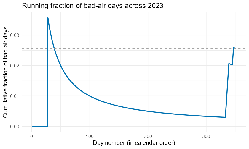

Running (cumulative) fraction of bad-air days at the Bakersfield-California monitor across the 351 measured days of 2023, in calendar order. One early exceedance (late January) sends the fraction up to about 0.036; with no more bad days it drifts down for months to a low near 0.003, before a December cluster pulls it back up to the overall 0.026 (dashed) by the right edge. Because the bad days are seasonally concentrated, the fraction approaches its final value from below, via a late-year rise, rather than settling smoothly — a reminder that the Law of Large Numbers governs the long-run total, not the moment-to-moment path when events cluster in time.

The second figure makes the conditional story visible: a histogram of daily PM2.5 with the 35 µg/m³ standard marked. Almost the whole distribution sits well below the line; the handful of exceedances are the right-tail outliers — and they are all winter days.

gf_histogram(~ daily_mean, data = day, bins = 25, fill = ok[5], color = "white") %>%
  gf_vline(xintercept = ~ 35, color = ok[2], linewidth = 1) %>%
  gf_labs(x = "Daily mean PM2.5 (µg/m³)",
          title = "Bakersfield daily PM2.5, 2023") %>%
  gf_theme(theme_minimal(base_size = 12))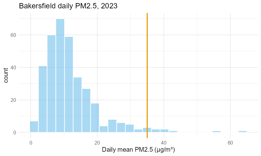

Distribution of daily mean PM2.5 (µg/m³) at the Bakersfield-California monitor in 2023, with the 35 µg/m³ health standard marked by a vertical line. The bulk of days are well below the standard; the few days to the right of the line are the 9 bad-air days, all of which occurred in winter.

9Durable skills¶

10Try it¶

Take these ideas to the interactive tools:

• Shiny — Statistics Explorer, “Sampling-Distribution Simulator” module. Resample the kern_airquality record to watch empirical probabilities form and stabilize; every action shows the equivalent R code you can copy. Launch the app with shiny::runApp("shiny-explorer") and open the simulator module.

• Jupyter — Lab 4: Probability by simulation (labs/lab04-probability.ipynb). A guided R-kernel notebook: estimate the bad-air probability, build the season-by-air-quality table, and run the “at least one bad day in 5” simulation end to end, then answer the reflection prompt on conditional reasoning.

11Chapter summary¶

• A probability $P(A)$ measures how likely an event $A$ is, on a 0-to-1 scale. The equally-likely view counts favorable outcomes over total outcomes; the long-run-frequency view is the fraction of repetitions in which $A$ happens, estimated from data as $\hat{P}(A) = n_A/n$.

• The axioms: $0 \le P(A) \le 1$, $P(S)=1$, and the complement rule $P(A^c) = 1 - P(A)$.

• Addition rule (for “or”): $P(A \cup B) = P(A) + P(B) - P(A \cap B)$; the overlap drops out only when $A$ and $B$ are disjoint.

• Conditional probability: $P(A \mid B) = P(A \cap B)/P(B)$ — the chance of $A$ within the world where $B$ is true. Rearranged, the multiplication rule is $P(A \cap B) = P(B)\,P(A \mid B)$.

• Independence means $P(A \mid B) = P(A)$, equivalently $P(A \cap B) = P(A)P(B)$. Multiply separate probabilities only when events are independent. Disjoint is not independent — disjoint events are maximally dependent.

• Simulation (sample, replicate, set.seed) estimates a probability by generating many repetitions and taking $M/N$; the Law of Large Numbers guarantees this converges to the true value. Always set.seed() for reproducibility.

• The Kern lesson: the overall 2.6% bad-air chance hides a 10.6% winter vs. 0% non-winter split — a vivid reminder that probabilities are conditional.

12FAQ¶

Q1. Is the 2.6% bad-air figure a “real” probability or just a sample fraction? It is an empirical probability — an estimate of the true long-run chance, based on 351 measured days. With more years of data the estimate would sharpen. It is exactly the kind of data-based probability we will turn into formal inference in Chapters 6 onward.

Q2. What’s the difference between $P(A \mid B)$ and $P(B \mid A)$? They answer different questions and are usually not equal. $P(\text{bad}\mid\text{winter}) = 9/85 \approx 0.106$ (“among winter days, how many are bad?”), while $P(\text{winter}\mid\text{bad}) = 9/9 = 1$ (“among bad days, how many are winter?”). Swapping the condition can flip the answer entirely — a classic source of error.

Q3. Can two events be both disjoint and independent? No (assuming both have positive probability). Disjoint means $P(A\cap B)=0$; independent means $P(A\cap B)=P(A)P(B)>0$. Those can’t both hold, so the two ideas are genuinely different — see the warning box in Section 5.

Q4. Why do I have to call set.seed() before simulating? Simulation uses random draws, so each run gives slightly different numbers. set.seed(k) fixes the random stream so anyone who reruns your code gets the identical result — essential for reproducible, checkable work. It does not bias the answer; it just makes it repeatable.

Q5. When can I multiply probabilities to get an “and”? Only when the events are independent, where $P(A\cap B)=P(A)P(B)$. If the events are dependent, use the general multiplication rule $P(A\cap B)=P(B)\,P(A\mid B)$ instead. Multiplying dependent probabilities is a frequent and serious mistake.

Q6. How many simulation repetitions are “enough”? More repetitions give a more precise estimate (the error shrinks roughly like $1/\sqrt{N}$). A few thousand is usually plenty for a rough probability; tens of thousands when you need two or three reliable decimal places. We will quantify this precisely in Chapter 6.

Q7. The histogram shows days above 35 — but you said summer never exceeds the standard. How? All the exceedances are winter days. Bakersfield’s PM2.5 problem is driven by winter temperature inversions, not summer heat. That is the whole point of Section 7.3: the risk is concentrated in one season, which a single annual probability completely obscures.

13Practice problems¶

Problems marked (sim) ask you to simulate in R; remember to set.seed(2200). Odd-numbered short answers appear in the appendix answer key; full worked solutions are in the instructor materials.

1. A fair coin is flipped once. What is $P(\text{heads})$, and what is the probability of not heads (the complement)?

2. A standard deck has 52 cards, 13 of them hearts. Find $P(\text{heart})$ for a single random draw.

3. Roll one fair die. Find $P(\text{roll} \le 2)$ and the probability of its complement.

4. In the Kern air-quality record, 9 of 351 Bakersfield-California days exceeded 35 µg/m³. Estimate $P(\text{bad air})$ and $P(\text{not bad air})$.

5. Events $A$ and $B$ are disjoint with $P(A)=0.3$ and $P(B)=0.25$. Find $P(A \cup B)$.

6. Events $C$ and $D$ have $P(C)=0.5$, $P(D)=0.4$, and $P(C \cap D)=0.2$. Find $P(C \cup D)$.

7. For the events in Problem 6, are $C$ and $D$ disjoint? Explain using $P(C \cap D)$.

8. A bag holds 4 red and 6 blue marbles. Draw one at random. Find $P(\text{red})$ and $P(\text{blue})$, and confirm they sum to 1.

9. Using the season-by-air-quality table (Winter: 85 days, 9 bad; Mar–Nov: 266 days, 0 bad), find $P(\text{bad} \mid \text{winter})$.

10. Using the same table, find $P(\text{winter} \mid \text{bad})$. Explain in one sentence why it differs from your answer to Problem 9.

11. Are “winter” and “bad air” independent for the Kern data? Justify with a numerical comparison of $P(\text{bad} \mid \text{winter})$ and $P(\text{bad})$.

12. A student has $P(\text{pass quiz}) = 0.8$ and $P(\text{pass exam}) = 0.7$, and the two are independent. Find $P(\text{pass both})$.

13. For the student in Problem 12, find $P(\text{pass at least one})$ using the addition rule.

14. Two fair dice are rolled. Using independence, find $P(\text{both show a } 6)$.

15. A test for a condition has $P(\text{positive} \mid \text{disease}) = 0.95$. Explain why this is not the same as $P(\text{disease} \mid \text{positive})$.

16. In a class, $P(\text{works a job}) = 0.6$, $P(\text{commutes}) = 0.5$, and $P(\text{works and commutes}) = 0.35$. Find $P(\text{works or commutes})$.

17. For Problem 16, find $P(\text{commutes} \mid \text{works})$ and state whether working and commuting appear independent.

18. Explain the difference between disjoint and independent events using a single concrete example of each.

19. (sim) Write R code using sample() and replicate() to estimate the probability that, in 5 days drawn at random (with replacement) from the Bakersfield record, at least one is a bad-air day. State your set.seed value.

20. (sim) Estimate $P(\text{sum} = 7)$ when rolling two fair dice by simulating 10,000 rolls. Compare your simulated value to the exact $6/36$.

21. A fair die is rolled. Let $A=\{\text{even}\}$ and $B=\{\text{at least }4\}$. Find $P(A \cap B)$ and $P(A \cup B)$ by listing outcomes.

22. For Problem 21, compute $P(A \mid B)$ and decide whether $A$ and $B$ are independent.

23. A company finds 2% of widgets are defective. Assuming defects are independent, find the probability that 3 randomly chosen widgets are all good.

24. (sim) Use simulation to estimate the probability in Problem 23 and compare it to the exact value 0.98³.

25. The complement rule says $P(A^c) = 1 - P(A)$. If $P(\text{at least one bad day in a week}) = 0.41$, what is $P(\text{no bad days all week})$?

26. Among 100 surveyed CSUB students, 40 commute and 25 of those commuters work. Find $P(\text{works} \mid \text{commutes})$ from these counts.

27. Explain, in one or two sentences, why $\hat{P}(A) = n_A/n$ from a sample is only an estimate of the true probability $P(A)$.

28. A weather app says “30% chance of rain.” Interpret this as a long-run frequency in one clear sentence.

29. Two events have $P(A) = 0.6$, $P(B) = 0.5$, and $P(A \cap B) = 0.30$. Are they independent? Show the check.

30. (sim) Resample the Bakersfield daily PM2.5 values 50,000 times and report the simulated $P(\text{daily mean} > 12)$ (the “moderate or worse” threshold); compare to the exact fraction in the data (128/351).

Glossary terms introduced in this chapter are collected in the book glossary (Appendix). Odd-numbered short answers appear in the answer-key appendix.

14Resumen en español¶