Inference for Proportions

# All chapter numbers come from executed code on real data — never typed by hand.
# data/processed/kern_calenviroscreen.csv is the chapter's primary dataset
# (CalEnviroScreen 4.0 indicators for Kern County census tracts; see its
# codebook in data/codebooks/kern_calenviroscreen.md).
suppressPackageStartupMessages({
  library(mosaic)   # favstats(), tally(), gf_*(), do() — the teaching stack
  library(BSDA)     # summary-statistic tests (used elsewhere in the course)
  library(ggplot2)  # used directly for the custom bar chart in §9.6
})
# Okabe–Ito colorblind-safe palette, used by this chapter's figure.
okabe_ito <- c("#0072B2", "#E69F00", "#009E73", "#CC79A7",
               "#56B4E9", "#D55E00", "#F0E442", "#999999")
knitr::opts_chunk$set(
  comment = "#>",
  collapse = TRUE,
  fig.width = 6.5,
  fig.height = 4,
  dpi = 150
)

1The Kern hook: counting burdened neighborhoods¶

California’s environmental-justice screening tool, CalEnviroScreen 4.0, scores every census tract in the state on cumulative pollution burden and population vulnerability, then reports each tract’s statewide percentile — the share of California tracts it scores at or above. By construction, exactly 25% of California tracts fall in the top quartile (percentile $\ge 75$). That is the statewide baseline: pick a California tract at random and there is a 1-in-4 chance it is “top-quartile burdened.”

Now ask the local question. Of the Kern County tracts with a reported score, what fraction land in that top statewide quartile?

ces    <- read.csv("data/processed/kern_calenviroscreen.csv")
scored <- subset(ces, !is.na(ces_percentile))     # keep only tracts that have a score
n_kern <- nrow(scored)                             # how many scored Kern tracts
x_kern <- sum(scored$ces_percentile >= 75)         # count in the statewide top quartile
phat   <- x_kern / n_kern                          # sample proportion
c(n = n_kern, successes = x_kern, phat = round(phat, 4))

Of the 147 scored Kern tracts, 73 are in the statewide top quartile — a sample proportion of $\hat p = 0.4966$, very close to half. (These values are computed above from data/processed/kern_calenviroscreen.csv; the dataset’s codebook records 151 Kern tracts, 4 with no composite score.) The statewide baseline is 0.25. Kern’s share is roughly double it.

But a sample proportion is not the whole story. Is $\hat p = 0.497$ convincingly different from the baseline 0.25, or could a county simply differ this much by chance? When the answer changes which neighborhoods get cleanup funding, you need more than a number — you need inference for a proportion. That is this whole chapter. By the end you will test exactly this claim and find the evidence is overwhelming: Kern really is more burdened than a typical California county.

2Learning objectives¶

After this chapter you will be able to:

1. (Apply) Construct a confidence interval for a single proportion and check the success/failure conditions.

2. (Apply) Conduct a one-sample $z$-test for a proportion and interpret the result in context.

3. (Apply) Conduct a two-proportion $z$-test and confidence interval, using the pooled standard error for the test.

4. (Analyze) Verify the independence and sample-size conditions for proportion inference and explain what goes wrong when they fail.

5. (Communicate) State a proportion conclusion — with its interval and its significance — for a non-technical audience.

Durable skills practiced: quantitative reasoning (inference for categorical outcomes) and quantitative communication (reporting a rate or a rate difference).

39.1 A proportion is a mean in disguise¶

3.1Intuition¶

A proportion is just the fraction of a group that has some trait: the share of tracts that are top-quartile burdened, the share of voters who say “yes,” the share of patients who recover. Code each unit as 1 for “has the trait” (a success) and 0 for “doesn’t” (a failure), and the proportion is simply the average of those 0/1 values. That is the key that unlocks everything: a proportion is a mean of 0/1 data, so all the sampling-distribution and confidence-interval ideas you already met for means carry straight over.

Because a proportion is a mean, the Central Limit Theorem from Chapter 6 applies. If your sample is large enough, the sampling distribution of $\hat p$ — the proportion you’d get from repeated samples — is approximately normal, centered at the true population proportion $p$, with a predictable spread. That normal shape is what lets us attach a $z$-score, a $p$-value, and an interval to a proportion.

3.2Formula¶

Let:

• $p$ = the population proportion (the unknown truth we want to learn about).

• $\hat p$ = the sample proportion (read “p-hat”), our estimate of $p$:

  $$\hat p = \frac{x}{n},$$

  where $x$ = the number of successes in the sample and $n$ = the sample size (number of observations).

The standard error of $\hat p$ — the typical distance between $\hat p$ and $p$ across repeated samples — is

Here $p(1-p)$ is the variance of a single 0/1 observation, and dividing by $n$ shrinks the spread as the sample grows (the familiar $\sqrt{n}$ effect from Chapter 6).

This normal approximation is trustworthy only when two conditions hold:

1. Independence. Observations are independent — typically guaranteed by a random sample drawn from a population at least 10 times the sample size (so sampling without replacement barely changes the odds).

2. Success–failure. There are at least 10 successes and 10 failures expected, so the sampling distribution is close enough to normal. Which counts you check depends on whether you are testing or estimating (we make this precise in Section 4 and Section 5).

3.3R¶

Base R gives you one function for both single- and two-proportion inference, prop.test(). For one proportion you pass the success count x, the sample size n, and the hypothesized value p = $p_0$; adding correct = FALSE turns off R’s continuity correction so the output lines up with the by-hand normal-approximation ($z$) formula you just met. Here it is on a tiny made-up poll of 540 “yes” out of 1000:

# 540 "yes" responses out of a 1000-person poll; test H0: p = 0.5.
prop.test(540, 1000, p = 0.5, correct = FALSE)

Read the printout top to bottom, and you can read every proportion test in the chapter:

• the title names the procedure (“1-sample proportions test without continuity correction”);

• X-squared = 6.4 is the test statistic. prop.test reports a chi-square value, and for a single proportion it is exactly the square of the $z$ you would compute by hand ($\sqrt{6.4} = 2.53$), on df = 1;

• p-value = 0.01141 is the two-sided $p$-value;

• the line alternative hypothesis: true p is not equal to 0.5 states $H_A$ (two-sided by default);

• the 95 percent confidence interval (here about 0.509 to 0.571) is R’s interval for $p$ — the Wilson score interval, a refined cousin of the Wald interval from Section 5;

• sample estimates: p = 0.54 is $\hat p = 540/1000$.

Once you can read one prop.test printout, you can read them all — every example below has the same shape.

49.2 Testing a single proportion¶

4.1Intuition¶

A hypothesis test for a proportion asks: if the population proportion were really some specific value $p_0$, would a sample as extreme as ours be surprising? We assume the null hypothesis $H_0: p = p_0$ is true, build the sampling distribution that $H_0$ predicts, locate our $\hat p$ on it, and ask how far out in the tail it sits. Far out (a small $p$-value) means our data would be unlikely if $H_0$ were true — evidence against $H_0$.

The subtle-but-important detail: when we test, we assume $H_0$ is true, so we compute the standard error using $p_0$, not $\hat p$. This is the null standard error. (When we estimate with a confidence interval in Section 5, we have no hypothesized value to lean on, so we use $\hat p$ instead. Same formula shape, different plug-in — keep them straight.)

4.2Formula¶

The one-proportion $z$-statistic is

where:

• $\hat p$ = sample proportion = $x/n$,

• $p_0$ = the hypothesized (null) proportion — the specific value $H_0$ claims,

• $n$ = sample size.

The denominator is the null standard error $SE_0 = \sqrt{p_0(1-p_0)/n}$. The $z$-statistic counts how many null standard errors separate $\hat p$ from $p_0$.

The $p$-value is the probability, under the standard normal curve, of a $z$-score at least as extreme as ours, in the direction(s) named by the alternative hypothesis $H_A$:

• $H_A: p \ne p_0$ (two-sided): $p\text{-value} = 2\,P(Z \ge |z|)$,

• $H_A: p > p_0$ (one-sided, greater): $p\text{-value} = P(Z \ge z)$,

• $H_A: p < p_0$ (one-sided, less): $p\text{-value} = P(Z \le z)$.

Compare the $p$-value to the significance level $\alpha$ (often 0.05). If $p\text{-value} < \alpha$, reject $H_0$; otherwise fail to reject $H_0$.

Test condition (success–failure under $H_0$): check $n p_0 \ge 10$ and $n(1-p_0) \ge 10$. Because the test assumes $H_0$, the expected counts use $p_0$.

4.3R¶

# Same poll: test H0: p = 0.5 against HA: p > 0.5 (is the "yes" share a majority?)
prop.test(540, 1000, p = 0.5, alternative = "greater", correct = FALSE)

Setting alternative = "greater" makes the test one-sided, and the $p$-value drops to 0.005706 — half the two-sided value, because all of the probability now sits in the upper tail. The object prop.test() returns also carries every number as a named field ($statistic, $p.value, $conf.int, $estimate), so a script or the Shiny app can read exact values with, say, prop.test(...)$p.value instead of copying them off the screen.

59.3 Estimating a single proportion with a confidence interval¶

5.1Intuition¶

A confidence interval (CI) for a proportion gives a range of plausible values for the true $p$, instead of a single test verdict. A 95% interval is built by a procedure that, across many samples, captures the true $p$ about 95% of the time. It answers “how big is it, and how sure are we?” rather than just “is it different from $p_0$?”

When estimating, we have no null value to assume, so we build the standard error from the data itself — the Wald standard error, using $\hat p$.

5.2Formula¶

A $C$-level confidence interval for $p$ is

where:

• $\hat p$ = sample proportion,

• $z^\star$ = the critical value — the normal cutoff leaving $(1-C)/2$ in each tail (for 95%, $z^\star = 1.96$),

• $\sqrt{\hat p(1-\hat p)/n}$ = the Wald standard error $SE_{\text{CI}}$ (note the $\hat p$, not $p_0$).

The piece after the ± is the margin of error, $\text{ME} = z^\star \cdot SE_{\text{CI}}$. A wider interval means more uncertainty; the interval narrows as $n$ grows and widens as the confidence level $C$ rises.

CI condition (success–failure from the data): check at least 10 observed successes ($x \ge 10$) and 10 observed failures ($n - x \ge 10$). Here the counts use $\hat p$, because no $H_0$ is assumed.

5.3R¶

prop.test() always prints a confidence interval alongside the test. To change the confidence level, set conf.level:

# A 90% CI for the "yes" share, from 540 of 1000.
prop.test(540, 1000, p = 0.5, conf.level = 0.90, correct = FALSE)

The 90 percent confidence interval line now reads about 0.514 to 0.566 — narrower than a 95% interval would be, because asking for less confidence buys a tighter interval. R computes this as a Wilson score interval; the hand formula below builds the closely related Wald interval $\hat p \pm z^\star SE$.

69.4 Comparing two proportions¶

6.1Intuition¶

Often the real question is a difference: is the success rate in group 1 different from the rate in group 2? Are Hispanic-majority Kern tracts more likely to be top-quartile burdened than other Kern tracts? Now we have two sample proportions, $\hat p_1$ and $\hat p_2$, and we care about $\hat p_1 - \hat p_2$.

The sampling distribution of that difference is again approximately normal (variances add when the two samples are independent), so the same $z$ machinery works — with one twist for the test. Under $H_0: p_1 = p_2$, both groups share one common proportion, so we estimate it by pooling all the successes from both groups. The test uses this pooled standard error; the confidence interval, which assumes no such equality, uses the unpooled standard error.

6.2Formula¶

Let group $i$ have $x_i$ successes in $n_i$ trials, so $\hat p_i = x_i / n_i$.

The pooled proportion combines both groups:

The two-proportion $z$-statistic (testing $H_0: p_1 - p_2 = 0$) is

where the denominator is the pooled standard error $SE_{\text{pool}}$. The intuition: if $H_0$ is true, both groups estimate the same $p$, so the best single estimate of it is the pooled one.

The confidence interval for $p_1 - p_2$ uses the unpooled standard error (each group keeps its own $\hat p_i$):

Conditions: independence within each group and between the two groups (separate random samples or a randomized experiment), plus the success–failure check in each group (at least 10 successes and 10 failures per group).

6.3R¶

For two proportions, prop.test() takes a vector of the two success counts and a vector of the two sample sizes. (Naming the entries, as below, just gives the data: line a tidy label.)

# Made-up trial: 45 of 100 recovered in group 1 vs 30 of 120 in group 2.
recovered <- c(group1 = 45, group2 = 30)
patients  <- c(group1 = 100, group2 = 120)
prop.test(recovered, patients, correct = FALSE)

The output now names two estimates — prop 1 = 0.45 and prop 2 = 0.25 — and the 95 percent confidence interval (about 0.075 to 0.325) is for their difference $p_1 - p_2$, built from the unpooled SE. The X-squared statistic (9.71, p-value = 0.001832) is computed from the pooled proportion behind the scenes, so both standard errors are at work in this single output even though only the difference is printed.

79.5 Worked examples¶

Each example follows the course rhythm: intuition $\rightarrow$ formula $\rightarrow$ computation $\rightarrow$ interpretation.

7.1Example 1 — Kern’s top-quartile share vs. the statewide baseline¶

(One-proportion test on the Kern CalEnviroScreen data.)

Intuition. By construction, 25% of California tracts are top-quartile burdened (percentile $\ge 75$). If Kern were a “typical” county, about a quarter of its tracts would land there. We saw in Section 1 that nearly half do. Is that gap real evidence of higher burden, or sampling noise? Test $H_0: p = 0.25$ against $H_A: p > 0.25$, where $p$ is the true proportion of Kern tracts that are top-quartile burdened.

Formula. One-proportion $z$ with the null SE: $z = (\hat p - p_0)\big/\sqrt{p_0(1-p_0)/n}$, with $p_0 = 0.25$.

Computation.

ces    <- read.csv("data/processed/kern_calenviroscreen.csv")
scored <- subset(ces, !is.na(ces_percentile))
x <- sum(scored$ces_percentile >= 75)
n <- nrow(scored)
prop.test(x, n, p = 0.25, alternative = "greater", correct = FALSE)

The success–failure check under $H_0$ uses $n p_0 = 147 \times 0.25 = 36.75$ and $n(1-p_0) = 110.25$, both well above 10, so the normal model is safe. From $x = 73$ of $n = 147$ scored tracts, prop.test reports the sample estimate $\hat p = 0.4966$ and X-squared = 47.68 — which is exactly the square of the by-hand statistic $z = 6.90$ ($\sqrt{47.68} = 6.90$) — with a one-sided p-value = 2.51e-12, astronomically small.

Interpretation. We reject $H_0$. There is overwhelming evidence that more than a quarter of Kern’s tracts are in the statewide top quartile of environmental burden — far more than a “typical” county would have. In plain terms: Kern County is disproportionately burdened, and the data say so loudly. (All values above are computed from data/processed/kern_calenviroscreen.csv.)

7.2Example 2 — A confidence interval for that share¶

(One-proportion CI on the same data.)

Intuition. A test told us Kern’s share exceeds 0.25. Estimation asks how big the share actually is. Build a 95% confidence interval for $p$.

Formula. $\hat p \pm z^\star \sqrt{\hat p(1-\hat p)/n}$ with $z^\star = 1.96$.

Computation.

prop.test(73, 147, p = 0.25, correct = FALSE)

By hand, $SE_{\text{CI}} = \sqrt{0.4966(1-0.4966)/147} = 0.0412$ and $\text{ME} = 1.96 \times 0.0412 = 0.0808$, giving the Wald interval $0.4966 \pm 0.0808 = (0.4158,\ 0.5774)$. R’s 95 percent confidence interval line prints 0.4169 to 0.5765 — the Wilson score interval, close to but not identical to the hand-computed Wald interval, because the two use slightly different arithmetic (the note in Section 5). For an intro course either is fine; just say which one you used.

Interpretation. We are 95% confident that between about 42% and 58% of Kern’s scored tracts are top-quartile burdened. The entire interval sits far above the statewide baseline of 25% — consistent with (and stronger than) the test in Example 1, because the whole plausible range excludes 0.25.

7.3Example 3 — Equity gap within Kern: two proportions¶

(Two-proportion test and CI on the Kern data.)

Intuition. Environmental-justice work asks who bears the burden. Split Kern’s scored tracts into Hispanic-majority tracts (hispanic_pct $\ge 50$) and not-majority tracts, and compare the proportion that are top-quartile burdened. Test $H_0: p_1 = p_2$ (no difference) against $H_A: p_1 \ne p_2$, where group 1 is Hispanic-majority and group 2 is not.

Formula. Two-proportion $z$ with the pooled SE for the test; unpooled SE for the CI of $p_1 - p_2$.

Computation.

ces <- read.csv("data/processed/kern_calenviroscreen.csv")
d   <- subset(ces, !is.na(ces_percentile) & !is.na(hispanic_pct))
# successes = top-quartile-burdened tracts; totals = all tracts, in each group
successes <- c(hispanic_majority = sum(d$ces_percentile >= 75 & d$hispanic_pct >= 50),
               not_majority      = sum(d$ces_percentile >= 75 & d$hispanic_pct <  50))
totals    <- c(hispanic_majority = sum(d$hispanic_pct >= 50),
               not_majority      = sum(d$hispanic_pct <  50))
prop.test(successes, totals, correct = FALSE)

Among 72 Hispanic-majority tracts, 53 are top-quartile burdened, so prop.test prints prop 1 = 0.7361; among 75 not-majority tracts, 20 are, giving prop 2 = 0.2667. Their difference is $\hat p_1 - \hat p_2 = 0.4694$. The pooled proportion $\hat p_{\text{pool}} = (53+20)/(72+75) = 0.4966$ drives the reported X-squared = 32.38, which is again the square of the by-hand $z = 5.69$ ($\sqrt{32.38} = 5.69$), with p-value = 1.27e-08.

Interpretation. We reject $H_0$: Hispanic-majority Kern tracts are far more likely to be top-quartile burdened than other Kern tracts. The 95 percent confidence interval for the difference prints as about $(0.327,\ 0.612)$ — i.e., the burdened share is between roughly 33 and 61 percentage points higher in Hispanic-majority tracts. (This interval is the unpooled one, exactly the standard error a CI for a difference should use.) This is a real, large equity gap in the data. (Note: CalEnviroScreen is observational, so this documents an association, not a cause — see the caution in Section 13.)

7.4Example 4 — Reading conditions: a poll that fails the check¶

(A conditions cautionary example.)

Intuition. Conditions are not paperwork — they decide whether the normal model applies at all. Suppose a pilot survey finds only 6 successes in 40 trials and you want to test $H_0: p = 0.5$.

Formula. Test success–failure under $H_0$: need $n p_0 \ge 10$ and $n(1-p_0) \ge 10$.

Computation. $n p_0 = 40 \times 0.5 = 20$ and $n(1-p_0) = 20$ — both exceed 10, so the test condition passes. But the CI condition uses the data: observed successes $x = 6 < 10$. The success–failure check for the interval fails.

prop.test(6, 40, p = 0.5, correct = FALSE)

Interpretation. With only 6 observed successes, any hand-computed Wald interval is unreliable — its normal approximation is shaky out in the tail. Helpfully, prop.test never uses the fragile Wald formula: the interval it prints (about 0.071 to 0.291) is the Wilson score interval, which stays sensible when a count is small, and is one of the recommended fixes here (an exact binomial or Agresti–Coull interval are others). Even so, the failed success–failure check is your early-warning signal. The lesson stands: always check the conditions before you trust the number — the software will still hand you an interval, condition or no condition.

89.6 Visualizing proportions¶

A bar chart of the two group proportions makes the equity gap from Example 3 immediate. We compute each group’s proportion, then plot.

ces <- read.csv("data/processed/kern_calenviroscreen.csv")
d   <- subset(ces, !is.na(ces_percentile) & !is.na(hispanic_pct))
d$group <- ifelse(d$hispanic_pct >= 50, "Hispanic-majority", "Not-majority")
# tapply(condition, group, mean) = the fraction TRUE (top-quartile) within each group
props <- tapply(d$ces_percentile >= 75, d$group, mean)
plot_df <- data.frame(group = names(props), proportion = as.numeric(props))

ggplot(plot_df, aes(x = group, y = proportion, fill = group)) +
  geom_col(width = 0.6) +
  geom_text(aes(label = sprintf("%.0f%%", 100 * proportion)),
            vjust = -0.4, size = 4.5) +
  scale_fill_manual(values = okabe_ito, guide = "none") +
  scale_y_continuous(limits = c(0, 0.85),
                     labels = function(x) sprintf("%.0f%%", 100 * x)) +
  labs(
    x = NULL,
    y = "Top-quartile burdened",
    title = "Kern environmental burden by tract demographics"
  ) +
  theme_minimal(base_size = 12) +
  theme(panel.grid.minor = element_blank(),
        plot.title = element_text(face = "bold"))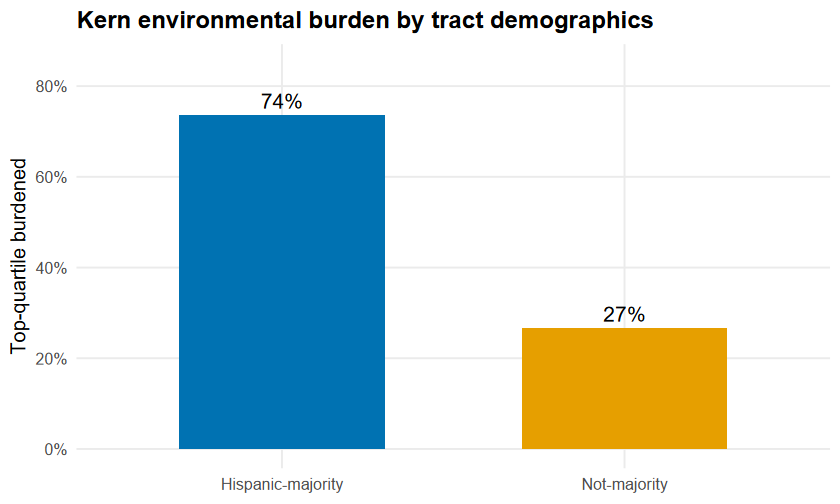

Proportion of Kern County census tracts in the statewide top quartile of environmental burden, by tract demographic group. Hispanic-majority tracts (74%) are far more likely to be top-quartile burdened than not-majority tracts (27%), a gap of about 47 percentage points.

The figure uses the Okabe–Ito colorblind-safe palette (blue and orange), labels both bars with their percentages, and is described in full by its alt text so a screen-reader user gets the same takeaway: a roughly 47-point gap.

9Durable-skill callouts¶

10Try it¶

• Shiny — Statistics Explorer, “One/Two-Sample Tests” module. Load kern_calenviroscreen, build the top-quartile indicator, and run the one- and two-proportion tests with point-and-click controls. The live code panel shows the matching prop.test() calls — copy them straight into your own script.

• Jupyter — Lab 9: Inference for Proportions (labs/lab09-proportions.ipynb). A guided walkthrough recomputes Examples 1–3 from the raw CSV, then asks you to test a proportion of your own choosing (e.g., the share of tracts above the drinking-water-index median) and write a one-paragraph conclusion.

119.7 Practice problems¶

Work each problem fully before checking. Odd-numbered answers are in Appendix: Answers; full worked solutions are in the instructor key. Unless stated otherwise, use $\alpha = 0.05$, two-sided alternatives, and 95% confidence. A calculator or R is allowed; keep full precision until the final step.

Conceptual.

1. Explain in one sentence why a proportion can be treated as the mean of a set of 0/1 values, and why that matters for inference.

2. State the two conditions required for the normal model to apply to a single proportion, and explain what each one protects against.

3. A test uses the standard error $\sqrt{p_0(1-p_0)/n}$ but a confidence interval uses $\sqrt{\hat p(1-\hat p)/n}$. Explain why the two procedures use different standard errors.

4. For a two-proportion test, why do we pool the two samples into a single proportion, while for the interval we do not?

5. A colleague says “the $p$-value is the probability that $H_0$ is true.” Give the correct interpretation of a $p$-value in one sentence.

One proportion — tests.

6. A national poll of $n = 1000$ adults finds $x = 540$ who favor a measure. Test $H_0: p = 0.5$ vs. $H_A: p \ne 0.5$. Report $\hat p$, $z$, the $p$-value, and your decision.

7. In a random sample of 50 CSUB students, 38 report owning a laptop. Test whether a majority own a laptop ($H_0: p = 0.5$ vs. $H_A: p > 0.5$). Report $z$ and the $p$-value.

8. A manufacturer claims at most 10% of its chips are defective. In a sample of 200 chips, 18 are defective. Test $H_0: p = 0.10$ vs. $H_A: p \ne 0.10$. What do you conclude?

9. A coin is flipped 40 times and lands heads 27 times. Test $H_0: p = 0.5$ vs. $H_A: p > 0.5$ at $\alpha = 0.05$. Is there evidence the coin is biased toward heads?

10. For the chip data in Problem 8, check the success–failure condition under $H_0$. Does the normal model apply?

One proportion — confidence intervals.

11. A survey of 400 commuters finds 120 use public transit. Construct a 95% confidence interval for the population proportion who use public transit.

12. Using the poll in Problem 6 ($x = 540$, $n = 1000$), construct and interpret a 95% confidence interval for $p$.

13. Explain how the width of a 95% CI for a proportion changes if (a) the sample size quadruples, and (b) the confidence level rises to 99%.

14. A pilot study finds 6 successes in 40 trials. Explain why you should not report an ordinary Wald 95% CI here, and what condition fails.

15. A pollster wants a 95% CI for a proportion with margin of error at most 0.03, and has no prior guess for $p$. Find the smallest sample size $n$ needed. (Hint: the worst case is $p = 0.5$.)

Two proportions.

16. A clinical trial reports 45 recoveries of 100 in the treatment group and 30 of 120 in the control group. Test $H_0: p_1 = p_2$ vs. $H_A: p_1 \ne p_2$ and report $z$, the $p$-value, and your decision.

17. For the trial in Problem 16, construct a 95% confidence interval for $p_1 - p_2$ and interpret it.

18. In County A, 210 of 300 sampled residents support a bond; in County B, 180 of 300 do. Is support different between the counties? Test at $\alpha = 0.05$.

19. For the counties in Problem 18, construct a 95% CI for the difference in support and state whether it is consistent with your test decision.

20. Explain why pooling is appropriate for the test in Problem 16 but not for the interval in Problem 17.

Kern CalEnviroScreen data (load it with ces <- read.csv("data/processed/kern_calenviroscreen.csv")).

21. Define a tract as “high-PM2.5” if its pm25 exceeds 12 µg/m³ (the older EPA annual standard). Compute the sample proportion of Kern tracts that are high-PM2.5, and test whether a majority of tracts exceed 12 µg/m³ ($H_0: p = 0.5$ vs. $H_A: p > 0.5$). Report $\hat p$, $z$, and your decision.

22. Construct a 95% confidence interval for the proportion of Kern tracts that are high-PM2.5 (as defined in Problem 21).

23. Define “high-PM2.5” instead as pm25 $> 9$ µg/m³ (the 2024 EPA standard). How does the sample proportion change, and what does that tell you about choosing a threshold?

24. Re-run Example 3’s two-proportion comparison but define the demographic groups by the poverty indicator instead (poverty $\ge$ its median vs. below). Report the two sample proportions and the $p$-value, and compare to the Hispanic-majority result.

25. In one or two sentences suitable for a county newsletter, report the result of Example 1 (Kern’s top-quartile share vs. the 25% baseline), including the estimate and a statement of significance, without using the word “$p$-value.”

Reasoning and communication.

26. A report states “the two recovery rates were not significantly different ($p = 0.21$).” Does this prove the treatments are equally effective? Explain.

27. Two studies estimate the same proportion. Study A: $\hat p = 0.40$, $n = 50$. Study B: $\hat p = 0.40$, $n = 500$. Without computing, which has the narrower 95% CI, and why?

28. A one-sided test gives $p = 0.03$. What would the two-sided $p$-value be for the same data, and which is appropriate if you had no prior direction in mind?

29. Explain why a statistically significant difference in proportions (very small $p$-value) is not automatically a practically important difference. Give a plausible example.

30. Using the Kern equity gap from Example 3, write two sentences a city council member could read aloud: one stating the estimated gap with its interval, and one stating the appropriate causal caution.

129.8 Chapter summary¶

• A proportion is the mean of 0/1 (success/failure) data, so the Central Limit Theorem makes the sampling distribution of $\hat p$ approximately normal — the basis for all proportion inference.

• One-proportion test: $z = (\hat p - p_0)/\sqrt{p_0(1-p_0)/n}$, using the null SE; compare the $p$-value to $\alpha$. Condition: $np_0 \ge 10$ and $n(1-p_0) \ge 10$.

• One-proportion CI: $\hat p \pm z^\star\sqrt{\hat p(1-\hat p)/n}$, using the Wald SE. Condition: at least 10 observed successes and 10 failures.

• Two-proportion test: pool the groups, $\hat p_{\text{pool}} = (x_1+x_2)/(n_1+n_2)$, and use the pooled SE; the CI for $p_1 - p_2$ uses the unpooled SE. Conditions: independence within and between groups, plus success–failure in each group.

• In R, prop.test() handles both one- and two-proportion inference: pass x, n, p = $p_0$ for one proportion, or a vector of the two success counts and a vector of the two totals for a comparison. Add correct = FALSE to match the by-hand ($z$/Wald) formulas; its X-squared statistic is the square of that $z$, and it prints a Wilson-score confidence interval.

• On the real Kern CalEnviroScreen data, ~50% of scored tracts are in the statewide top quartile of burden (vs. a 25% baseline, $z \approx 6.9$), and Hispanic-majority tracts are ~47 percentage points more likely to be top-quartile burdened ($z \approx 5.7$) — large, significant, and an association, not a proven cause.

139.9 FAQ¶

Q1. When do I use the null ($p_0$) standard error and when the sample ($\hat p$) one? Use the null SE for a hypothesis test (you are assuming $H_0$, so plug in $p_0$); use the Wald ($\hat p$) SE for a confidence interval (no $H_0$ to assume). For two proportions, the test pools; the interval does not.

Q2. My test rejects $H_0$ but the difference looks tiny. What gives? With a large $n$, even a small, practically meaningless difference can be statistically significant. Always pair the $p$-value with the confidence interval so you can judge whether the size of the effect matters, not just whether it is nonzero (see Problem 29).

Q3. The success–failure condition fails — now what? The normal approximation is unreliable. Report the limitation and use an exact or adjusted method instead (for one proportion, an exact binomial test or the Agresti–Coull interval; these are introduced as tools you can reach for, not required formulas in this course).

Q4. Does the Kern equity result mean Hispanic demographics cause higher burden? No. CalEnviroScreen data are observational: tracts were not randomly assigned their demographics. The two-proportion test documents a strong association between tract demographics and environmental burden — a real, important pattern — but causation would require ruling out confounders (industrial siting history, housing policy, income). Report associations honestly and resist causal language (Chapter 1’s scope-of-inference lesson applies here).

Q5. One-sided or two-sided? Choose the alternative before seeing the data, based on the question. Use one-sided only when a direction is genuinely the only one of interest (“is it a majority?”); otherwise use two-sided. Never switch to one-sided after peeking to make a result “significant.”

Q6. Why does my 95% CI sometimes include values the test rejected, or vice versa? For two proportions, the test uses the pooled SE and the CI uses the unpooled SE, so they can occasionally disagree at the boundary. They usually agree; when they don’t, it is because they answer slightly different questions with slightly different standard errors. Trust the procedure that matches your goal (test for “is there a difference,” CI for “how big”).

Q7. What’s the smallest sample I can use? There is no single number, but the success–failure condition is the practical gate: you want at least 10 successes and 10 failures (per group, for two proportions). Below that, switch to exact methods.

14Resumen en español¶