Inference for Means

# Chapter-wide R setup. Every numeric value printed in this chapter's prose was
# independently recomputed in Python (pandas/scipy) from the same curated CSVs
# in data/processed/ and matches the R output below to rounding. The datasets
# are: kern_crops_sim (SIMULATED — see its codebook), fitness_tracker_sim
# (SIMULATED), and nhanes_subset (REAL teaching sample, not survey-weighted).
suppressPackageStartupMessages({
  library(mosaic)   # t.test(y ~ g, data=), gf_*(), favstats() — the teaching stack
  library(BSDA)     # tsum.test(): a t-test straight from summary statistics
})
# Okabe–Ito colorblind-safe palette, used by this chapter's figures.
okabe_ito <- c("#0072B2", "#E69F00", "#009E73", "#CC79A7",
               "#56B4E9", "#D55E00", "#F0E442", "#999999")
set.seed(2200)      # reproducibility for any resampling demo
knitr::opts_chunk$set(collapse = TRUE, comment = "#>", fig.align = "center")

1A Kern County opener: did almond yield really change?¶

Kern County is one of the most productive farm counties in the United States, and almonds are one of its signature crops. Suppose a grower looks back at the last nine crop years and asks a simple question: “Is our typical almond yield really about one ton per acre, or is it drifting?”

We can put a number on the “typical” yield. Using the curated teaching dataset kern_crops_sim, the mean almond yield per acre across the nine crop years 2015–2023 is 1.0359 tons per acre (dataset-derived from kern_crops_sim, variable yield_per_acre; see the codebook data/codebooks/kern_crops_sim.md).

crops  <- read.csv("data/processed/kern_crops_sim.csv")
almond <- subset(crops, commodity == "ALMONDS")
mean(~yield_per_acre, data = almond)   # dataset-derived: 1.0359 tons/acre

That sample mean of 1.0359 is close to one ton per acre — but it is built from only nine years, and yields wobble from year to year with the weather. So the honest question is not “is 1.0359 exactly 1?” (it never will be), but: is the gap between 1.0359 and 1 large enough to be real, or is it the kind of wobble we would expect from nine noisy years even if the true long-run mean were exactly 1? That is a question about a population mean, and this chapter is the tool for it: the t-test family.

2Learning objectives¶

By the end of this chapter you will be able to:

1. (Apply) Conduct a one-sample $t$-test and confidence interval for a mean, and state the conditions the $t$-distribution requires.

2. (Apply) Conduct a paired $t$-test by analyzing the differences, and explain when pairing is the right design.

3. (Apply) Conduct a two-sample $t$-test and confidence interval for a difference of means.

4. (Analyze) Choose between a paired and a two-sample procedure for a given study design, and justify the choice.

5. (Evaluate) Assess the normality and independence conditions and judge how robust the $t$ procedures are when those conditions bend.

Durable skills this chapter builds: quantitative reasoning (QR) and critical thinking (CT).

Before this chapter you should be comfortable with confidence intervals (Chapter 7) and the logic of hypothesis testing — null/alternative hypotheses, p-values, and significance level (Chapter 8).

3Why a t and not a z? The intuition¶

3.1Intuition¶

In Chapter 6 you learned that a sample mean $\bar{x}$ varies from sample to sample, and the size of that variation — the standard error — is the population standard deviation divided by $\sqrt{n}$. To turn $\bar{x}$ into a test we standardize it: we measure how many standard errors $\bar{x}$ sits away from the value we are testing.

There is one practical snag. The standard error needs the population standard deviation $\sigma$, and we almost never know it. We have to estimate it with the sample standard deviation $s$. That substitution adds a second source of uncertainty: not only is $\bar{x}$ noisy, but our ruler for measuring its noise is itself estimated from the same small sample.

The fix is to use a distribution that is a little more spread out than the normal — heavier in the tails — to honestly reflect that extra uncertainty. That distribution is Student’s $t$. With few observations the $t$ is noticeably wider than the normal; as the sample grows, the estimate of $s$ settles down and the $t$ becomes indistinguishable from the normal. The amount of extra spread is controlled by one number, the degrees of freedom.

3.2Formula¶

The one-sample $t$ statistic is

where

• $\bar{x}$ = the sample mean (the average of your data),

• $\mu_0$ (read “mu-naught”) = the hypothesized population mean — the value in the null hypothesis,

• $s$ = the sample standard deviation (your estimate of the spread),

• $n$ = the sample size (number of observations),

• $s/\sqrt{n}$ = the standard error of the mean, written $\mathrm{SE}$,

• and we compare $t$ to a $t$-distribution with $df = n - 1$ degrees of freedom. ($df$, “degrees of freedom,” is the single number that sets how heavy the tails are; here it is one less than the sample size.)

The two-sided p-value is the probability, if $H_0$ were true, of a $t$ at least as far from zero as the one we observed.

The confidence interval for $\mu$ inverts the same machinery:

where $t^{\star}_{df}$ (read “t-star”) is the critical value: the point on the $t$-distribution with $df$ degrees of freedom that puts the chosen confidence level (say 95%) in the middle.

3.3R¶

In R, the one-sample procedure is t.test(). With mosaic you can write it in the formula form t.test(~variable, data = , mu = ), where mu is the value $\mu_0$ you are testing against. Its output is compact — the statistic, degrees of freedom, p-value, confidence interval, and sample mean — which we unpack line by line in Worked Example 1:

# (Run for real in @ch10-sec-ex1 below; shown here only to introduce the function.)
t.test(~yield_per_acre, data = almond, mu = 1.0)

4The one-sample t-test¶

4.1Intuition¶

Use a one-sample $t$-test when you have one group of measurements and a specific number you want to compare its mean against — a standard, a target, a historical value, a claim. “Is the mean wait time under 15 minutes?” “Is the average fill weight 12 ounces?” “Is the typical almond yield one ton per acre?”

4.2Formula¶

Exactly Equation and Equation above. The hypotheses are

(or $<$ / $>$ for a one-sided test). Conditions for the $t$ procedure:

1. Independence — observations are independent (a random sample, or fewer than 10% of a finite population).

2. Normality / sample size — the data come from a roughly normal population, or the sample is large enough ($n \ge 30$ is the usual rule of thumb) for the Central Limit Theorem to make $\bar{x}$ approximately normal. For small $n$, check that the data are roughly symmetric with no extreme outliers.

4.3Worked Example 1 — almond yield vs. one ton per acre (Kern data)¶

Intuition. Back to the opener. We have nine yearly almond yields and one benchmark, $\mu_0 = 1$ ton per acre. One group, one number to compare against: a one-sample $t$-test.

Formula. $H_0:\ \mu = 1$ vs. $H_A:\ \mu \ne 1$, using Equation with $df = 9 - 1 = 8$.

Computation.

t.test(~yield_per_acre, data = almond, mu = 1.0)

The pieces, recomputed and dataset-derived from kern_crops_sim: $\bar{x} = 1.0359$ tons/acre (R’s mean of x), $s = 0.0765$, $n = 9$, so $\mathrm{SE} = 0.0765/\sqrt{9} = 0.0255$ and

R prints exactly this: t = 1.4082, df = 8, a two-sided p-value = 0.1967, and a 95 percent confidence interval of 0.977 to 1.095 tons per acre.

Interpretation. Because $p = 0.197 \ge 0.05$, we fail to reject $H_0$. There is not enough evidence to say the long-run mean almond yield differs from one ton per acre. The confidence interval tells the same story a richer way: one ton per acre sits comfortably inside (0.977, 1.095), so it remains a plausible value for the true mean. The 0.0359 gap we saw in the opener is exactly the kind of wobble nine noisy years can produce on their own.

4.4A picture of the data¶

A small sample earns a look before a test. Are the nine yields roughly symmetric with no wild outlier? Image shows they are.

xbar <- mean(~yield_per_acre, data = almond)
gf_histogram(~yield_per_acre, data = almond, bins = 6,
             fill = okabe_ito[1], color = "white") %>%
  gf_vline(xintercept = ~xbar, color = okabe_ito[4],
           linetype = "dashed", linewidth = 0.8) %>%
  gf_labs(
    x = "Almond yield (tons per acre), 2015–2023 — SIMULATED",
    y = "Number of crop years",
    title = "Almond yield per acre is roughly symmetric (kern_crops_sim)",
    subtitle = paste0("Dashed line = mean = ", signif(xbar, 4))
  )

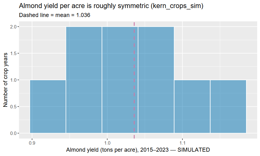
Nine almond yields cluster between about 0.9 and 1.2 tons per acre with no extreme outlier, so the t-procedure’s normality condition is reasonable for this small sample.

5The paired t-test¶

5.1Intuition¶

Sometimes two columns of numbers are naturally matched, one-to-one: a before-and-after measurement on the same person, the left and right hand of the same athlete, a 2015 and a 2023 value for the same crop. When the data come in matched pairs, the smart move is to subtract within each pair and analyze the single column of differences. Pairing strips away the variation between subjects (some crops are just bigger than others) so the variation within a pair (did this crop grow or shrink?) stands out on its own.

A paired $t$-test is therefore not a new test at all — it is a one-sample $t$-test run on the differences, testing whether their mean is zero.

5.2Formula¶

Let $d_i = (\text{value 1})_i - (\text{value 2})_i$ be the difference for pair $i$. Then with

• $\bar{d}$ = the mean of the differences,

• $s_d$ = the standard deviation of the differences,

• $n$ = the number of pairs,

the statistic is

where $\mu_0$ is the hypothesized mean difference (almost always 0: “no change”). Everything else — p-value, confidence interval — is the one-sample machinery applied to the $d_i$.

5.3Worked Example 2 — did Kern crop acreage shift from 2015 to 2023? (Kern data)¶

Intuition. For each of eight Kern commodities we have its harvested acres in 2015 and again in 2023. The two columns are matched by commodity — almonds to almonds, cotton to cotton — and they share the same unit (acres). That is a paired design. We ask: across these crops, did acreage change on average?

Formula. $d_i = (\text{acres}_{2023})_i - (\text{acres}_{2015})_i$ for each commodity; $H_0:\ \mu_d = 0$ vs. $H_A:\ \mu_d \ne 0$, via Equation with $df = 8 - 1 = 7$.

Computation. First reshape the data so each commodity is one row with a 2015 column and a 2023 column (that plumbing is hidden below; the resulting paired table is shown):

# (Reshaping plumbing hidden — it aligns each commodity's 2015 and 2023 acreage
# into one row. The resulting paired table, one row per crop, is what matters:)
yr2015 <- crops[crops$year == 2015, c("commodity", "harvested_acres")]
yr2023 <- crops[crops$year == 2023, c("commodity", "harvested_acres")]
names(yr2015)[2] <- "acres_2015"
names(yr2023)[2] <- "acres_2023"
paired_crops <- merge(yr2015, yr2023, by = "commodity")
paired_crops

Now the paired test. Subtract within each pair to get one column of differences, then run a one-sample $t$-test on that column — that is the paired test:

paired_crops$diff <- paired_crops$acres_2023 - paired_crops$acres_2015
t.test(~diff, data = paired_crops, mu = 0)

Dataset-derived from kern_crops_sim: the differences have mean $\bar{d} = 8193.25$ acres (R’s mean of x) and $s_d = 22{,}080$ acres over $n = 8$ pairs, so $\mathrm{SE} = 7806.5$. R prints t = 1.0495, df = 7, a p-value = 0.3288, and a 95 percent confidence interval for the mean change of (-10,266, 26,653) acres.

Interpretation. Some crops grew a lot (pistachios, almonds) and others shrank (cotton). On average, acreage rose by about 8,200 acres per crop. But with only eight crops and huge swings from one crop to the next, that average is swamped by noise. Since $p = 0.329 \ge 0.05$, we fail to reject $H_0$: there is no average shift we can detect. The interval includes zero, which confirms that “no change” is still a plausible answer. Notice the payoff of the design: by pairing on commodity, we never had to pretend a carrot field and a cotton field were interchangeable — we only ever compared each crop to itself.

6The two-sample t-test¶

6.1Intuition¶

Now suppose the two groups are separate sets of subjects with no natural pairing: a treatment group and a control group, men and women, two different fields. We cannot subtract within pairs because there are no pairs. Instead we compare the two group means directly and ask whether their difference is bigger than sampling noise would explain.

6.2Formula¶

With sample means $\bar{x}_1, \bar{x}_2$, sample standard deviations $s_1, s_2$, and sample sizes $n_1, n_2$, the Welch two-sample $t$ statistic (which does not assume the two groups have equal variance) is

where

• $\bar{x}_1, \bar{x}_2$ = the two sample means,

• $s_1, s_2$ = the two sample standard deviations,

• $n_1, n_2$ = the two sample sizes,

• $\mu_0$ = the hypothesized difference under $H_0$ (usually 0),

• and the denominator is the standard error of the difference, $\mathrm{SE}$.

The hypotheses are $H_0:\ \mu_1 - \mu_2 = 0$ vs. $H_A:\ \mu_1 - \mu_2 \ne 0$. The degrees of freedom for Welch’s $t$ come from a longer formula that R works out for you, so you never have to compute it by hand; it is usually not a whole number. R’s t.test() uses Welch by default because it is safer than assuming the two groups have equal variance.

6.3Worked Example 3 — did the activity program raise daily steps? (randomized study)¶

Intuition. The fitness_tracker_sim dataset records a hypothetical randomized study: 200 people were randomly assigned to a treatment group (an 8-week activity-coaching program) or a control group, and their mean daily steps were recorded. Random assignment makes the two groups independent and comparable, so a two-sample $t$-test is exactly right.

fit <- read.csv("data/processed/fitness_tracker_sim.csv")
# List treatment first so the reported difference reads treatment − control
# (otherwise R orders the groups alphabetically and would report control first).
fit$group <- factor(fit$group, levels = c("treatment", "control"))
tally(~group, data = fit)   # 100 treatment, 100 control

Formula. $H_0:\ \mu_{\text{treat}} - \mu_{\text{control}} = 0$ vs. $H_A:\ \mu_{\text{treat}} - \mu_{\text{control}} \ne 0$, via Equation.

Computation. Pass the numeric response and the grouping column:

t.test(steps ~ group, data = fit)

Dataset-derived from fitness_tracker_sim: R lists mean in group treatment = 8112.9 steps/day and mean in group control = 7170.9, a difference of 942.0 steps/day, with $\mathrm{SE} = 302.2$, so

matching R’s t = 3.1169, df = 197.98, a p-value = 0.0021, and a 95 percent confidence interval for the difference of (346, 1538) steps per day. (Because we put treatment first in the setup, R reports the difference as treatment − control, so it comes out positive.)

Interpretation. Because $p = 0.0021 < 0.05$, we reject $H_0$: the program group walked significantly more. The confidence interval (346, 1538) excludes zero and is entirely positive, so we are 95% confident the program adds somewhere between about 350 and 1,500 daily steps on average — a difference that is both statistically detectable and, for a step count, practically meaningful.

Image shows the two groups side by side: the treatment box sits visibly higher, but with plenty of overlap — which is why we needed the test to confirm the shift is more than noise.

gf_boxplot(steps ~ group, data = fit, fill = ~group, width = 0.6) %>%
  gf_refine(scale_fill_manual(
    values = c(control = okabe_ito[1], treatment = okabe_ito[2]), guide = "none")) %>%
  gf_labs(
    x = "Group (randomized assignment)",
    y = "Mean daily steps — SIMULATED",
    title = "Daily steps by group (fitness_tracker_sim)"
  )

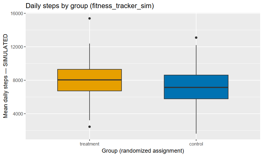
Side-by-side boxplots of mean daily steps for the control and treatment groups in fitness_tracker_sim. The treatment median sits above the control median, with overlapping spreads — consistent with the significant but moderate difference the t-test found.

6.4Worked Example 4 — a “no difference” result, and reading it honestly (NHANES)¶

Intuition. Not every test ends in rejection, and a non-significant result is information, not failure. The nhanes_subset dataset is a real CDC teaching sample of body measurements. Adult female height in the United States is often quoted as about 162 cm. Does this sample’s mean agree?

Formula. One group (adult women), one benchmark $\mu_0 = 162$ cm: $H_0:\ \mu = 162$ vs. $H_A:\ \mu \ne 162$, via Equation.

Computation.

nhanes <- read.csv("data/processed/nhanes_subset.csv")
women  <- subset(nhanes, sex == "female" & age >= 20)
t.test(~height_cm, data = women, mu = 162)

Dataset-derived from nhanes_subset: R reports mean of x $= 162.04$ cm over $n = 3658$ non-missing observations (the subset holds 3,683 rows, but t.test drops the 25 with a missing height), t = 0.355, df = 3657, a p-value = 0.7225, and a 95 percent confidence interval of (161.81, 162.28) cm.

Interpretation. With $p = 0.72$, we fail to reject $H_0$ — the sample mean of 162.04 cm is fully consistent with a population mean of 162 cm. Notice two teaching points. First, the huge sample ($n = 3658$) makes the interval very narrow (less than half a centimeter wide), so this is a precise “no difference,” not a vague one. Second, “fail to reject” never means “we proved $\mu = 162$ exactly”; it means 162 is among the many plausible values the data support.

7Choosing the right procedure¶

The hardest part of this chapter is not the arithmetic — R does that — it is matching the test to the design. Use this decision flow:

1. How many groups of measurements?

   • One group, compared to a fixed number $\rightarrow$ one-sample $t$ (t.test(~y, data = D, mu = )).

   • Two groups $\rightarrow$ go to step 2.

2. Are the two groups matched one-to-one?

   • Yes — each value in group 1 is paired with a specific value in group 2 (before/after, twins, same unit at two times) $\rightarrow$ paired $t$ (t.test(~diff, data = D) on the within-pair differences).

   • No — the two groups are separate, independent sets of subjects $\rightarrow$ two-sample $t$ (t.test(y ~ g, data = D)).

For the full menu of every test in the course — not just the three in this chapter — see the book’s which-test decision guide in the appendix; it routes you from “what kind of data do I have?” to the right procedure.

8Try it¶

• Shiny — Statistics Explorer, “One/Two-Sample Tests” module. Load fitness_tracker_sim or kern_crops_sim, pick a numeric variable and a group, and run the $t$-test interactively. Every click shows the exact R code it ran, so the app and this chapter teach identical syntax. Launch the app from shiny-explorer/ (shiny::runApp("shiny-explorer")) and open the One/Two-Sample Tests tab.

• Jupyter lab — labs/lab10-inference-for-means.ipynb. A guided, runnable notebook (R kernel) that walks through the one-sample and two-sample t.test() forms on these datasets, with starter-code exercises and a reflection prompt. On JupyterHub it loads the data by relative path; locally, open it from the labs/ folder.

9Practice problems¶

Problems marked [Kern] use a Kern-anchored dataset. Odd-numbered problems have short answers in the book’s Answers appendix; full worked solutions are in the instructor key. Unless stated otherwise, use $\alpha = 0.05$ and a two-sided alternative, and assume the $t$ conditions hold well enough to proceed.

1. [Kern] In your own words, explain why the almond-yield analysis in Section 4.3 used a one-sample $t$-test rather than a two-sample test. What are the “one sample” and the “one number” here?

2. State the three members of the $t$-test family covered in this chapter and, in one sentence each, the design that calls for each one.

3. A one-sample $t$-test on $n = 16$ observations gives $\bar{x} = 48$, $s = 8$, and tests $H_0:\ \mu = 50$. Compute the standard error and the $t$ statistic by hand (show Equation plugged in). State the degrees of freedom.

4. Explain in plain language why the $t$-distribution is wider than the normal distribution, and what happens to that extra width as $n$ grows.

5. [Kern] Using kern_crops_sim, write the R call with t.test() that tests whether the mean pistachio yield per acre differs from 1.2 tons per acre. You do not need to run it — just write the correct one line of code.

6. A paired study measures blood pressure before and after a treatment on the same 12 patients. Why is a paired $t$-test more appropriate here than a two-sample $t$-test? What does pairing “remove”?

7. For the steps analysis in Section 6.3, the 95% confidence interval for the difference was (346, 1538) steps. Interpret this interval in one sentence for a campus wellness coordinator who has never taken statistics.

8. True or false, and explain: “A non-significant result ($p = 0.72$) proves the two means are equal.” Use Section 6.4 to ground your answer.

9. [Kern] A grower claims the mean table-grape yield in kern_crops_sim is 7 tons per acre. The nine yearly values have $\bar{x} = 7.31$ and $s = 0.20$. Compute the $t$ statistic for $H_0:\ \mu = 7$ and state whether you would reject at $\alpha = 0.05$ (the critical value is about $t^\star = 2.31$).

10. Decide paired vs. two-sample for each design, and say why: (a) left-hand vs. right-hand grip strength of 30 athletes; (b) test scores of 25 students taught online vs. 25 different students taught in person; (c) a city’s monthly rainfall this year vs. last year, month-matched.

11. [Kern] Using fitness_tracker_sim, write the t.test() call that compares resting heart rate (resting_hr) between the treatment and control groups.

12. A two-sample (Welch) $t$-test reports $df = 41.7$. Explain why the degrees of freedom are not a whole number, and why we use Welch’s version by default.

13. Sketch (describe) what the side-by-side boxplots would look like for a two-sample comparison that is not significant. How does the overlap compare to Image?

14. A paired $t$-test on $n = 10$ pairs gives $\bar{d} = 3.0$, $s_d = 5.0$. Test $H_0:\ \mu_d = 0$: compute $\mathrm{SE}$, the $t$ statistic, and the $df$.

15. [Kern] Explain why this chapter labels its kern_crops_sim numbers as simulated and refuses to present them as facts about real Kern almond farming. What would change if a real USDA NASS key were registered?

16. Explain the link between the test decision and the confidence interval: if a 95% CI for $\mu$ is $(12.4, 18.1)$, what is the result of the two-sided test of $H_0:\ \mu = 15$ at $\alpha = 0.05$? Of $H_0:\ \mu = 20$?

17. [Kern] Using fitness_tracker_sim, the mean sleep (sleep_hours) was 7.11 (treatment) vs. 6.83 (control), with a two-sample $t = 1.99$, $df \approx 196$, $p = 0.048$. State the conclusion at $\alpha = 0.05$, and explain why you should be cautious calling a $p = 0.048$ result a big effect.

18. A colleague runs a two-sample $t$-test on data that are actually paired (before/after on the same people). Will ignoring the pairing tend to make the standard error too big or too small, and how could that change the conclusion?

19. [Kern] For the almond one-sample test in Section 4.3 ($t = 1.41$, $df = 8$, $p = 0.197$), suppose a grower says “the p-value is above 0.05, so the mean yield is definitely exactly one ton per acre.” Correct this statement.

20. List the two conditions a one-sample $t$-test requires, and for the nine-value almond sample, explain how Image helps you check the normality condition.

21. A study compares mean wait times at two clinics: clinic A ($n_1 = 40$, $\bar{x}_1 = 22$ min, $s_1 = 6$) and clinic B ($n_2 = 35$, $\bar{x}_2 = 19$ min, $s_2 = 5$). Set up $H_0$ and $H_A$ and compute the standard error of the difference using Equation’s denominator.

22. Why does a larger sample size make a confidence interval narrower? Tie your answer to the $\sqrt{n}$ in the standard error.

23. [Kern] In Section 5.3 the paired test on crop acreage gave $p = 0.329$. Explain how it is possible that several individual crops changed acreage a lot, yet the average change was not statistically significant.

24. Give one real-world example from your own major or job of (a) a one-sample $t$ question, (b) a paired $t$ question, and (c) a two-sample $t$ question.

25. A one-sided one-sample test of $H_0:\ \mu = 100$ vs. $H_A:\ \mu > 100$ gives $t = 1.80$ on $df = 24$. Without software, is the one-sided p-value larger or smaller than the two-sided p-value for the same $t$? By what factor?

10Chapter summary¶

• Inference for a mean uses the $t$-distribution, not the normal, because we estimate the standard deviation $s$ from the sample. The $t$ is wider in the tails (set by $df = n-1$) and converges to the normal as $n$ grows.

• The one-sample $t$-test (t.test(~y, data = D, mu = )) compares one group’s mean to a fixed value $\mu_0$ via $t = (\bar{x}-\mu_0)/(s/\sqrt{n})$.

• The paired $t$-test (t.test(~diff, data = D) on the within-pair differences) is a one-sample test on the differences of matched pairs; use it when the two columns are matched one-to-one.

• The two-sample (Welch) $t$-test (t.test(y ~ g, data = D)) compares the means of two independent groups via Equation and does not assume equal variances.

• The design dictates the test. Decide paired vs. two-sample from how the data were collected, never from which p-value you prefer.

• The decision and the confidence interval always agree, and the interval — reported in real units — is usually the more useful summary for a stakeholder.

11FAQ¶

Q1. When can I use a $z$-test for a mean instead of a $t$-test? In practice, almost never. A $z$-test for a mean requires knowing the population standard deviation $\sigma$, which you essentially never do. Whenever you estimate the spread with the sample $s$ — i.e., always — use the $t$-test. With large $n$ the two give nearly identical answers anyway, because the $t$ converges to the normal.

Q2. My sample is small ($n < 30$). Can I still use a $t$-test? Yes, if the data look roughly symmetric with no extreme outliers (so the normality condition is believable). The almond example ($n = 9$) is fine because Image shows a single rough mound. If a small sample is badly skewed or has outliers, the $t$ procedure is unreliable and you would turn to a randomization/bootstrap method (Chapters 7–8) instead.

Q3. What is the difference between the paired test and just running two groups? The paired test — t.test(~diff, data = D) on a column of within-pair differences — needs the two columns to be the same length and matched row-by-row, and it tests whether the mean difference is zero. The two-group form t.test(y ~ g, data = D) treats the samples as independent. They answer different questions and give different standard errors; pick based on the design (Section 7).

Q4. Why is the Welch degrees-of-freedom not a whole number? Welch’s method adjusts the degrees of freedom to account for the two groups possibly having different spreads and sizes, and that adjustment usually lands on a fractional value rather than a whole number. R reports it exactly. You never compute it by hand — just read it from the output and trust it.

Q5. The confidence interval includes 0. What does that mean? For a difference of means, an interval that includes 0 means “no difference” is a plausible value — equivalent to failing to reject $H_0$ at the matching significance level. In Section 5.3 the acreage-change interval $(-10{,}266, 26{,}653)$ includes 0, so we could not conclude the average acreage changed.

Q6. Does a significant result ($p < 0.05$) mean the effect is large or important? No. Significance means the effect is detectable given the sample size, not that it is big. Always read the confidence interval in real units to judge whether the effect matters practically. A tiny, useless difference can be “significant” with a large enough sample, and a meaningful difference can be non-significant in a small one.

Q7. Can I use these tests on the simulated Kern data and report the numbers as real? No — and this is a rule, not a preference. The _sim datasets are clearly labeled synthetic; their numbers are for learning the method. The moment you have real USDA NASS data (register a free key), rerun the identical code and report those numbers instead. The code does not change; only the data behind it does.

12Glossary¶

New terms introduced in this chapter are collected in the book’s Glossary appendix. They include: Student’s $t$-distribution, degrees of freedom, standard error of the mean, one-sample $t$-test, paired $t$-test, two-sample (Welch) $t$-test, mean difference, and critical value $t^\star$.

13Resumen en español¶