The Cost Model
MATH 3219: what a generated token cost on this machine, and what that number leaves out
Every week of this course ends with the same fourth question: what did that cost? This appendix is where the answer is kept, so that a chapter can cite a figure in one line and you can come here to find out exactly how it was obtained.
It is one measurement, made on one machine, with a meter that sees part of the machine and not all of it. The point of this appendix is the boundary between the part it saw and the part it did not. Read Part 2 before you quote anything from Part 1.
Two files hold every measured number below.
| File | Written by | Holds |
|---|---|---|
lab/out/theme_s_energy.json | lab/theme_s_energy.py | power, speed and energy per token for the three models |
lab/out/lab4_size_ladder.json | lab/lab4_size_ladder.py | accuracy, memory footprint and timings for the same three models |
Anything else on this page is arithmetic on those two files, and the arithmetic is shown so you can check it.
1. What we measured
1.1 The machine
One laptop, one GPU, one evening.
| Item | Value |
|---|---|
| GPU | NVIDIA RTX 3500 Ada Generation Laptop GPU |
| Enforced board power limit | 55 W |
| Idle board power | 13.8 W, the median of 246 samples taken over 5 seconds with nothing running |
| Decoding | greedy |
| Prompt | Explain why the sky is blue, in three sentences. |
| Token budget | max_new_tokens = 120 |
| Instrument | NVML board power, sampled at about 50 Hz across the generation window |
Three terms, defined here because the rest of the appendix leans on them.
A watt (W) is a rate: one joule of energy every second. A joule (J) is the energy
itself. A watt-hour (Wh) is one watt sustained for an hour, which is 3,600 J. Board
power is what the whole graphics card draws from the machine, the chip and its memory and its
voltage regulators together. NVML is the NVIDIA Management Library, the measurement
interface the graphics driver exposes; the command-line tool nvidia-smi is a thin wrapper
around it, so both read the same sensor.
Greedy decoding means the model always emits its single highest-probability next token, with no randomness anywhere. That matters here for a reason that has nothing to do with energy: it makes the run repeatable. Sampling would give a different sentence each time and therefore a different number of tokens, and you would not be able to tell whether a change in the energy figure came from the model or from the dice.
1.2 The method, step by step
Read the GPU’s idle board power for 5 seconds with nothing running, and take the median of the samples rather than the mean. One spike from a background process moves a mean and does not move a median.
Load the model at FP16 onto the GPU.
Generate 8 tokens and throw them away. The first generation after a model loads pays for CUDA kernel compilation, a one-time cost that has nothing to do with what a token costs in steady state. Skip this warm-up and every model looks worse than it is.
Start a background thread that records board power every 20 ms, which is about 50 readings a second.
Generate, greedily, up to 120 new tokens. Record the wall-clock time and the number of tokens that actually came out.
Stop the sampler. Take the mean of the power samples across the generation window, multiply by elapsed seconds to get total joules, and divide by tokens generated.
Step 6 is where the two reported columns come from.
1.3 The two formulas
Let be mean board power in watts over the generation window, the idle board power in watts, and the throughput in tokens per second. Energy per token is
because watts are joules per second, and dividing joules per second by tokens per second leaves joules per token. The marginal, or “above idle”, figure subtracts the power the card would have drawn anyway:
To turn either into watt-hours per thousand tokens, multiply by 1,000 and divide by 3,600.
1.4 The table
Table 1:What one generated token cost on this machine. Greedy decoding, FP16 weights, one run per model.
| Model | Parameters | tok/s | Mean board power (W) | J per token | J per token above idle | Wh per 1,000 tokens | Power samples |
|---|---|---|---|---|---|---|---|
| Qwen2.5-0.5B | 494,032,768 | 27.7 | 21.3 | 0.767 | 0.268 | 0.213 | 151 |
| Qwen2.5-1.5B | 1,543,714,304 | 24.2 | 27.4 | 1.133 | 0.561 | 0.315 | 244 |
| Qwen2.5-3B | 3,085,938,688 | 15.6 | 30.2 | 1.941 | 1.052 | 0.539 | 278 |
Two things move at once as the model grows, and both push the same way. The larger model draws more power and produces tokens more slowly. Energy per token is power divided by speed, so it rises faster than either factor on its own. From the 0.5B to the 3B, mean power rose by a factor of while speed fell by a factor of . The product of those two factors is the ratio of the two energy figures, .
1.5 Why the “above idle” column exists
A powered-on GPU draws 13.834 W on this machine whether or not a model is running. While the 0.5B model generates, the card averages 21.254 W. So of the 0.767 J that one token cost,
is the card being switched on, and 0.268 J is the arithmetic the model actually did. The same share is 50.5% for the 1.5B and 45.8% for the 3B. Because energy per token is power divided by a speed that does not depend on the idle draw, the idle share of the power is exactly the idle share of the energy per token.
That is why the two columns answer different questions, and why you have to say which one you mean.
| Question you are asking | Column to use | 0.5B to 3B |
|---|---|---|
| What did this generation cost, on a machine switched on to do it? | J per token | 2.53× |
| What did choosing the larger model add, given the machine was on anyway? | J per token above idle | 3.93× |
Neither is wrong. The total column is right if the machine was turned on for this job and turned off afterwards. The marginal column is right if the machine was going to be on regardless and you are deciding which model to point at it, which is the situation a student with one laptop is actually in. Report both, and name the one your conclusion rests on.
2. The limits
This is not a disclaimer at the foot of the page. It is the part of the appendix that decides whether the numbers above may be used for a given argument.
2.1 GPU board power only. No CPU, no RAM, no motherboard, no power-supply conversion losses, no display, no cooling fans. The processor in this laptop was running the Python process that drove the generation, and none of that energy is in the table.
2.2 One laptop GPU, under Windows WDDM, at a 55 W cap. A desktop card, a server card, or this same chip at a different enforced power limit will give a different number. These figures describe this hardware. Do not carry them to other hardware, and do not let anyone carry them to yours.
2.3 One run, one prompt, greedy, so . There is no replication here, therefore no standard error and no interval, and none is printed. This is a measurement, not a benchmark. A benchmark would repeat the run across prompts and across sessions and report the spread. Chapter 12 is where that distinction grows teeth.
2.4 The three runs generated different numbers of tokens: 85, 120 and 88. Two of the models reached an end-of-sequence token before the 120-token budget ran out. Every figure in the table is per token, so this does not bias the comparison, but it is the reason the wall-clock totals are not comparable directly.
2.5 A datacenter figure would be larger, not smaller. A hosted model runs in a facility whose cooling, lighting and power distribution all draw energy on top of the server itself. The ratio of total facility energy to computing-equipment energy is called PUE, power usage effectiveness, and a cloud figure has to be multiplied by it. There is also networking, and there are machines kept powered and idle so that your request does not wait. None of that is in this table, because none of it applied: the model ran on the machine in front of us.
2.6 The memory figures in Part 3 are weights only. They count the parameters and nothing else. Running a model also needs room for the activations and for the cache of past tokens, which grows as the conversation lengthens. The weight figure is a floor.
3. The join that makes Theme S quantitative
Part 1 measured energy. Chapter 13’s scoring procedure measured accuracy. They were run separately, by different scripts, on the same three models. Joining them is what turns “small models are more sustainable” from a slogan into a calculation you can check.
3.1 The accuracy side, with its warning attached
From lab/out/lab4_size_ladder.json, scored by the rotation-debiased procedure of Chapter 13 on
the 20-question bank:
| Model | Accuracy (rotation-debiased) | Standard error | Answers consistent under rotation |
|---|---|---|---|
| Qwen2.5-0.5B | 15.0% | 0.080 | 1 of 20 |
| Qwen2.5-1.5B | 70.0% | 0.102 | 13 of 20 |
| Qwen2.5-3B | 95.0% | 0.049 | 18 of 20 |
3.2 The two steps up the ladder
| Step | Accuracy gained | Energy per token | Above-idle energy per token |
|---|---|---|---|
| 0.5B to 1.5B | +55 points | ×1.48 | ×2.10 |
| 1.5B to 3B | +25 points | ×1.71 | ×1.87 |
The arithmetic, so you can check it:
Divide accuracy gained by the energy multiple to get accuracy points bought per unit of extra energy:
The first step buys 2.55 times as much accuracy per unit of energy as the second. That is diminishing returns, measured rather than asserted.
Now do it again with the marginal column, because Part 1.5 said you must name your accounting and this is the test of whether the choice mattered:
The first step is now 1.97 times better instead of 2.55 times better. The size of the effect changes; the direction does not. The conclusion survives either way of counting. A conclusion that survives a change of accounting is worth more than one that needs a particular column to stand up.
3.3 The access line, in bytes
FP16 stores each parameter in 16 bits, which is 2 bytes. So the weights occupy exactly twice the parameter count in bytes.
| Model | Parameters | Parameters × 2 bytes | Weights |
|---|---|---|---|
| Qwen2.5-0.5B | 494,032,768 | 988,065,536 bytes | 0.99 GB |
| Qwen2.5-1.5B | 1,543,714,304 | 3,087,428,608 bytes | 3.09 GB |
| Qwen2.5-3B | 3,085,938,688 | 6,171,877,376 bytes | 6.17 GB |
A note on units, because this is the kind of thing that quietly breaks an argument. Above, GB means 109 bytes. A graphics card advertised as 4 GB holds 4 GiB, which is bytes. Converted into the card’s own units, the 1.5B weights are 2.88 GiB and the 3B weights are 5.75 GiB.
Either convention gives the same verdict, and it is not close in either: a 4 GB student laptop GPU fits the 1.5B and does not fit the 3B. Since Part 2.6 warned that weights are a floor, the 3B is further out of reach than 6.17 GB by itself suggests.
3.4 The thesis, stated as arithmetic
The environmental factor and the access factor were measured independently, on different quantities, in different units. They point at the same model.
The energy argument says the first step up the ladder is the bargain and the second is not, by a factor of about two whichever column you use.
The access argument says the 1.5B is the largest of the three that fits a modest machine.
A model small enough to be cheap to run is a model cheap enough to be widely available. These are not two findings that happen to agree. They are one variable seen twice, because both are driven by parameter count. Theme S asks you to analyse the connectedness between two factors that influence sustainability and justice. Here you can compute it rather than be told it.
One more comparison, built only from the measured numbers, to set the scale of an inference run. Generating 1,000 tokens on the 1.5B costs 0.315 Wh. Leaving this same GPU powered on and idle for one hour costs 13.834 Wh, which is 43.9 times as much. On the evidence of this one machine, the energy question for local inference is at least as much about how long the hardware stays switched on as about which model you point at it. That is a statement about this laptop, and Part 2.5 is the reason it does not transfer to a datacenter.
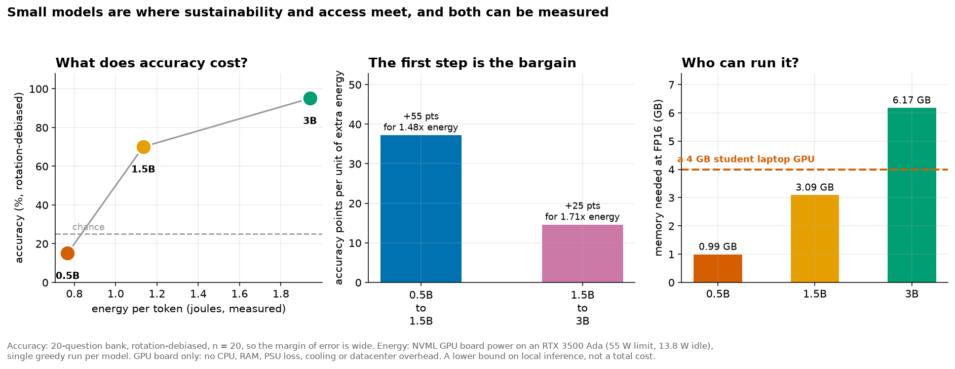
The Theme S join. Accuracy from lab4_size_ladder.json, energy from theme_s_energy.json,
memory computed as two bytes per parameter. Accuracy rests on 20 questions, so its margin of
error is wide; energy rests on one greedy run per model and covers GPU board power only.
4. How to measure it yourself
This is the procedure in Lab 1. Your numbers will not match the table in Part 1, and they are not meant to: different hardware, different power limit, different driver. What must match is the method and the honesty of the reporting.
4.1 If you have an NVIDIA GPU
Install the management-library binding once:
uv pip install nvidia-ml-pyYou can confirm the sensor is live from a terminal before writing any Python. This prints one reading and exits:
nvidia-smi --query-gpu=name,power.draw,memory.total --format=csvThen the measurement. This is the core of lab/theme_s_energy.py, reduced to the part that
matters:
import pynvml, time, statistics

pynvml.nvmlInit()
h = pynvml.nvmlDeviceGetHandleByIndex(0)

# Runs in a background thread while the model generates.
samples = []
while generating:
    samples.append(pynvml.nvmlDeviceGetPowerUsage(h) / 1000.0)   # mW to W
    time.sleep(0.02)                                             # about 50 Hz

mean_w    = statistics.mean(samples)
total_j   = mean_w * elapsed_seconds
j_per_tok = total_j / tokens_generated
Four things you must do, in this order, or the number is wrong:
Take the idle baseline first, with the model not loaded and nothing else running, and record the median.
Warm up. Generate a few tokens and discard them before you start the sampler.
Use greedy decoding and a fixed token budget, and record how many tokens you actually got.
Sample across the generation window only. Starting the sampler before the model loads averages loading into generating and understates the per-token figure.
4.2 Why the idle baseline is not optional
Without it you cannot separate a machine that is working from a machine that is merely on, and Part 1.5 showed that on this hardware the difference is most of the number: 65.1% of the 0.5B’s per-token energy was the card being powered up. Report an energy figure with no idle baseline beside it and your reader has no way to tell whether they are looking at the cost of the model or the cost of the laptop.
Take the baseline on the same day, on the same machine, in the same power mode. A laptop on battery saver and the same laptop plugged in are, for this purpose, two different instruments.
4.3 If you do not have an NVIDIA GPU
You are not locked out of Lab 1. Three routes, in descending order of how much they tell you.
Route A, a wall-plug energy meter. A meter between the charger and the outlet measures more of the machine than NVML does, not less: processor, memory, screen, charging losses, all of it. Take an idle baseline the same way, with the machine on and nothing generating, and subtract. Then label your result whole-system power and write one sentence saying it is not comparable to a GPU-board figure. That sentence earns marks. Holding two numbers that cannot be compared, and saying so, is the skill this lab is actually teaching.
Route B, measure the two legs that need no meter. Throughput in tokens per second needs a clock and a token count. Memory needs the parameter count and the two-bytes-per-parameter rule of Part 3.3. Those two legs carry the access argument on their own, and the access argument is half of Theme S.
Route C, pair up. Work with someone who has an NVIDIA card, and record whose machine produced which row. Provenance is part of the deliverable. A table that does not say where each row came from is not finished.
5. What we did not measure, and will not guess
Three real costs sit outside this appendix. The course names them, leaves them blank, and says why.
| Cost | Our figure | Why it is blank |
|---|---|---|
| Training energy | [to be measured] | We did not train these models. Qwen2.5 was trained on someone else’s hardware, before we met it, with no meter of ours attached. |
| Water for cooling | [to be measured] | This laptop is air cooled and consumed no water directly. The electricity behind the wall socket has a water footprint that we did not measure and cannot infer from a power reading. |
| Embodied carbon of manufacture | [to be measured] | The emissions from making this GPU, this laptop and their packaging were incurred before the first line of the lab ran. Nothing in lab/ can reach them. |
All three matter. For training energy in particular, it is not obvious whether training or a lifetime of inference is the larger share of what a model costs the world. We do not know which is larger for these models, and this appendix does not pretend to.
5.1 Published estimates exist, and we did not copy them into our tables
These three papers were fetched and checked on 12 September 2026. They are where a capstone on this question should start.
Strubell, E., Ganesh, A. and McCallum, A. (2019), Energy and Policy Considerations for Deep Learning in NLP, arXiv:1906.02243. https://
arxiv .org /abs /1906 .02243 Luccioni, A. S., Viguier, S. and Ligozat, A.-L. (2022), Estimating the Carbon Footprint of BLOOM, a 176B Parameter Language Model, arXiv:2211.02001. https://
arxiv .org /abs /2211 .02001 Li, P., Yang, J., Islam, M. A. and Ren, S. (2023), Making AI Less “Thirsty”: Uncovering and Addressing the Secret Water Footprint of AI Models, arXiv:2304.03271. https://
arxiv .org /abs /2304 .03271
Not one of their figures appears in any table on this page, and that is deliberate. A number lifted out of a paper and set in a column beside 0.767 J starts, within about one reading, to look like the same kind of object: something this course measured. It is not. Those papers estimated different quantities, on different hardware, for different models, by methods you would have to read before you could defend the number in a seminar.
5.2 What to do with them in your own work
Cite them as someone else’s estimate. Name the paper, name the quantity they estimated, and name the method. Keep the figure out of any table that holds your own measurements, or put it in a separate table with a column headed “source”. If a reader cannot tell at a glance which numbers you produced and which you borrowed, the table is not honest yet, however accurate every entry in it happens to be.
5.3 The refusal is the lesson
This book’s policy is that we never publish a number we did not compute. Applied to energy, that policy is cheap: we owned the meter. Applied to training energy, water and embodied carbon, it costs us three rows in a table, and it is the same policy either way. A rule you only follow when it is free is not a rule.
The capstone asks you for a resource-cost accounting. A blank marked [to be measured], with one sentence on what instrument or record would fill it, scores better in this course than a confident figure you cannot source. Anyone can produce the confident figure. Knowing which of your numbers you are entitled to is the harder skill, and it is the one being graded.
6. Provenance of every number on this page
Table 2:Where each figure came from. Nothing on this page originates anywhere else.
| Figures | Source |
|---|---|
| Idle 13.834 W, mean power, tok/s, J per token, J per token above idle, Wh per 1,000 tokens, power-sample counts, tokens generated (85 / 120 / 88) | lab/out/theme_s_energy.json, written by lab/theme_s_energy.py |
GPU name, 55 W enforced power limit, prompt, max_new_tokens, the exclusions list | the _meta block of lab/out/theme_s_energy.json |
| Idle baseline as the median of 246 samples over 5 seconds | _research/00-lab-verified-findings.md, section 9 |
| Accuracy 15.0 / 70.0 / 95.0%, standard errors, rotation consistency, parameter counts, FP16 sizes | lab/out/lab4_size_ladder.json, written by lab/lab4_size_ladder.py |
| McNemar’s exact | lab/out/we7_paired.json, written by lab/we7_paired_comparison.py; see Chapter 13 |
| Ratios 1.42, 1.78, 1.48, 1.71, 2.53, 1.87, 2.10, 3.93; shares 65.1%, 50.5%, 45.8%; 37.2 against 14.6 and 26.2 against 13.3; 2.55 and 1.97; 43.9; the byte counts and GiB conversions | arithmetic on the two JSON files above, shown in full in Parts 1 and 3 |
| Training energy, water for cooling, embodied carbon | not measured. See Part 5 |