Capstone
Chapter 15. One question, one honest number, one cost, and the rubric that pays for all three
Chapter 15. One question, one honest number, one cost, and the rubric that pays for all three
What you need before this chapter
This chapter introduces no new mathematics. Every formula in it appeared earlier in the book. What is new is that you now have to choose which ones to use, on a question you picked yourself, and defend the choice in front of people.
From this book, in order of how much you will lean on it:
| Chapter | What you take from it | Where it appears in your capstone |
|---|---|---|
| Chapter 11, Can a model take a test? | accuracy as a proportion, and how to pull an answer out of a model | your headline number |
| Chapter 12, Is that score real? | the standard error, the 95 per cent interval, the bootstrap | the interval that goes beside the headline number |
| Chapter 13, Measure your measurement | three scoring procedures, rotation, the paired comparison, McNemar | your method section, and your comparison if you make one |
| Chapter 7, Quantization | bytes per weight, energy per token, the access line | your resource-cost accounting |
| Chapter 14, Bias in the benchmark | subgroup breakdowns | your limitations section |
From the Math Toolkit, these sections and no others:
Section 12, proportions and what “out of” means, because your headline number is a proportion.
Section 9, square roots, because the standard error has one in it.
Section 11, percentages, decimals and fractions and percentage points, because the difference between “35 per cent” and “35 percentage points” is a graded distinction.
Section 19, inequalities and interval notation, because you will be writing intervals like all semester.
Section 10, sigma notation, because the grading formula in Section 6 of this chapter is a sum.
Section 16, rounding and significant figures, because rounding at the wrong moment is the most common arithmetic slip in a capstone report.
Section 2, subscripts and Section 4, the fraction bar, if the notation in any formula below stops you.
An honest warning about sequencing. If Chapter 12 has not clicked yet, go back to it before Milestone 3 in Week 12. The interval is worth 30 of the 150 points on your final submission, and those are the points students most often lose. There is no way to earn them without Chapter 12.
Setup
Run this cell once at the top of every notebook you write for your capstone. Everything below in this chapter assumes it has already run.
# Chapter 15 setup. One import per line, each with a comment saying what it is for.

import json                       # reads the .json result files that this course's labs wrote
import math                       # square roots and rounding up, for standard errors and sample sizes
import numpy                      # arrays and averages, for per-question score vectors
import matplotlib.pyplot as plt   # bar charts and interval plots for your capstone report

# The colourblind-safe Okabe-Ito colours this book uses in every figure.
# Never let colour be the only thing carrying meaning in a chart. Label it too.
okabe_ito_blue = "#0072B2"
okabe_ito_orange = "#E69F00"
okabe_ito_green = "#009E73"
okabe_ito_vermillion = "#D55E00"
okabe_ito_grey = "#999999"

# Figure defaults, so every chart in your report comes out the same size and weight.
plt.rcParams["figure.figsize"] = (7.0, 4.2)
plt.rcParams["figure.dpi"] = 150
plt.rcParams["font.size"] = 11

# The folder that holds every measured result in this course. Your own results go here too.
lab_output_folder = "lab/out"

# The multiplier for a 95 per cent interval. It comes from the normal distribution and it is
# the same number in every interval you will compute this semester.
z_for_95_percent = 1.96

print("setup complete")
setup completeWhy this chapter exists
Picture a Tuesday evening board meeting for one of the school districts in Bakersfield. A company is presenting a tutoring product built on a language model. The slide on the screen says the product answers student questions with 94 per cent accuracy.
Nobody in the room asks what that number is.
That scene is made up. It has not happened in exactly that form, and the 94 per cent is invented for the example, not quoted from anyone. But you have sat through something close to it, and by now you know four questions that would take that slide apart, and you know them because you measured them yourself:
Ninety-four per cent of what? On which questions? Written by whom?
Out of how many? In Chapter 12 a model scored 5 out of 20 on a statistics quiz, which is 25.0 per cent, and the honest 95 per cent interval around that score ran from 6.0 per cent to 44.0 per cent. Twenty questions cannot settle anything.
Scored how? In Chapter 13 one model, on one set of twenty questions, scored 25.0 per cent, 35.0 per cent or 15.0 per cent depending only on which of three defensible scoring procedures you used. The naive procedure was measuring the model’s fondness for the letter A, which it picked on 16 of 20 questions.
What did it cost, and who can run it? The 3B model in this course spends 1.941 joules of electricity per token it writes, from
lab/out/theme_s_energy.json, which is , so 2.53 times what the 0.5B model spends. It needs 6.17 gigabytes of memory, fromlab/out/lab4_size_ladder.json, which does not fit on a 4 gigabyte student laptop.
Being able to take the slide apart is a good skill. It is not the skill this course is for.
The capstone asks for the harder thing: produce the better number yourself. Pick a model, pose a question that can be answered, fix a procedure before you run it, run it, report what you found with an interval around it, and account for what the run cost in energy and in access. Then stand up and explain it in three minutes to forty-four classmates who know exactly which questions to ask you.
That is the whole assignment. It is worth 200 points of the 1000 in this course, and , so per cent of your grade. It is the single largest item on the syllabus.
Learning objectives
By the end of this chapter you will be able to:
Write a capstone question that names a model, a measurable quantity, a fixed procedure and a sample size, and explain why a question missing any one of those cannot be answered.
Compute the margin of error for a planned evaluation, and use it in reverse to work out how many questions your question bank needs before you build it.
Choose between a paired and an unpaired analysis when you compare two models, and compute the paired interval by hand from a per-question score vector.
Produce a resource-cost accounting for your own project in joules, watt-hours and gigabytes, and state the limits of that measurement in the same paragraph.
Score your own draft against the four-criterion rubric before you submit it, including the arithmetic of what a missing interval costs you.
This lesson at a glance
A capstone result is three things, never one: an estimate, an interval, and a cost. A number without the other two is not finished.
The question decides everything else. A good question names the quantity, the procedure and the sample size in advance; a weak one hides all three behind a word like “better”.
The rubric pays for honesty, in points. Two rubric items, worth of the 150 points on your final submission, are about reporting uncertainty, and a bare accuracy number scores zero on both.
The work is spread across five milestones, from Week 9 to Week 14, so that nothing about your project is a surprise in Week 15, least of all to you.
The vocabulary of this chapter
Every term below is defined here before any numbered section of the chapter uses it. Nothing in this table assumes you met it earlier, including the few terms carried over from Chapters 12 and 13.
| Term | What it means, in one line |
|---|---|
| capstone | the final project of this course: one question, one honest evaluation, one report, one three-minute talk |
| estimand | the true quantity you wish you knew, which you will never see directly |
| estimate | the number your run actually produced, which stands in for the estimand |
| headline number | the single number a reader will remember from your report, such as “70 per cent” |
| standard error | how much your estimate would bounce around if you drew a fresh question bank of the same size |
| margin of error | how far your estimate might sit from the estimand, as a plus-or-minus |
| interval | the pair of numbers you get by subtracting and adding the margin of error |
| Wald interval | the interval you get from the standard error of a proportion times 1.96, the one this chapter computes |
| p-value | the probability of seeing a result at least this lopsided if the two things being compared were really equal |
| statistically significant | the convention that a p-value below 0.05 is small enough to report a difference as real |
| question bank | the fixed set of questions you score a model on |
| preregistration | writing down your procedure, in full, before you run it |
| pilot run | a small trial run, done early, whose only job is to prove the code works end to end |
| forward pass | one trip of one prompt through the model, producing one set of scores |
| paired design | giving both models the same questions, so each question is answered twice |
| discordant pair | a question where the two models disagree: one right, one wrong |
| resource-cost accounting | a table of what your project consumed: energy, memory, time |
| joule (J) | the unit of energy; one watt drawn for one second is one joule |
| watt-hour (Wh) | the energy of one watt kept running for one hour, which is 3,600 joules |
| rubric | the table of criteria your work is graded against, published in advance |
| criterion | one row of the rubric, with its own point value |
| milestone | a dated checkpoint, worth points, that proves the project is moving |
| lightning talk | a very short presentation with a hard time limit and a fixed slide count |
| reproducible report | a report whose every number can be regenerated by running the code beside it |
1. What the capstone asks of you
1.1 Intuition
Think about the last time somebody told you a price. “It’s about forty dollars.” You did not write that down and treat it as exact. You heard it as a range, and you knew without thinking that the real number might be thirty-five or forty-five, and that if the real number turned out to be four hundred you had been misled rather than rounded to.
A measurement works the same way and people forget it, because a measurement arrives dressed as a single number. “The model scored 70 per cent.” That sentence sounds complete. It is not complete, and the reason is the same reason “about forty dollars” is not a receipt: you have been handed one number where two are needed.
Here is why a second number is unavoidable. You did not test the model on every question in the world. You tested it on the questions you had. If you had written a different set of questions, of the same kind and the same difficulty, the model would have scored something else. Your question bank is a sample, and a score computed on a sample is a number that would have come out differently if the sample had come out differently. Chapter 12 measured exactly this: on twenty questions, a score of 25.0 per cent came with a 95 per cent interval running from 6.0 per cent to 44.0 per cent.
So a capstone result has a fixed shape, and the shape has three slots.
The three examples below come from one imagined project. The counts in them, 39 right out of 60
and 60,000 tokens, are made up for practice, so that you can check every step. The energy
rate of 1.133345 joules per token and the memory figure of 3.09 gigabytes are measured, from
lab/out/theme_s_energy.json and lab/out/lab4_size_ladder.json. Section 4.4 works the whole
thing through with every step shown.
Slot one, the estimate. The number your run produced. “39 out of 60, which is 65.0 per cent.”
Slot two, the interval. How far that estimate might sit from the truth. “95 per cent interval: 52.9 per cent to 77.1 per cent.”
Slot three, the cost. What the run consumed. “The full run generated 60,000 tokens on Qwen2.5-1.5B-Instruct, an estimated 18.889 watt-hours at the measured rate of 1.133345 joules per token, on a model needing 3.09 gigabytes of memory.”
Notice the six decimals on that energy rate. Quote the rate at the precision your arithmetic actually used, so a reader can reproduce your watt-hours from your own sentence. Rounding the rate to 1.133 first gives 18.883 watt-hours instead of 18.889, and a grader who checks your arithmetic will find the gap.
A report that fills all three slots is finished. A report that fills one of them is a rumour with a decimal point in it. The rubric in Section 6 pays for all three, and it pays most for the second, because the second is the one everyone drops.
1.2 The mathematics
The headline number in almost every capstone in this course is a proportion: how many the model got right, out of how many you asked.
Formula 1: the sample proportion, your headline number
In words. Count how many questions the model got right. Divide that by how many questions you asked. That fraction is your headline number.
The formula.
The symbols.
| Symbol | How to say it out loud | What it means |
|---|---|---|
| “p hat” | your estimate of the model’s accuracy, a number between 0 and 1 | |
| “p” | the letter chosen for a proportion; the hat is what makes it an estimate rather than the truth | |
| the hat, | “hat” | a mark meaning “estimated from data”, never “measured exactly” |
| “x” | how many questions the model answered correctly, a whole number | |
| “n” | how many questions you asked, a whole number | |
| the fraction bar | “divided by” | divide the number on top by the number underneath. The Math Toolkit builds the fraction bar from zero. |
| “divided by” | the division sign. It does the same job as the fraction bar, written on one line, and the worked examples below use it. | |
| “equals” | the thing on the left and the thing on the right are the same number |
Out loud. “P hat equals x over n, which is the number the model got right divided by the number of questions you asked.”
Worked, with made-up small numbers. A bank of 40 questions. The model answered 18 correctly.
Step 1, write down the two numbers. , .
Step 2, divide.
Step 3, turn the decimal into a percentage by multiplying by 100. A percentage is a number “out of a hundred”, so multiplying by 100 is the whole conversion, and the Math Toolkit works several of these both ways. , so the model scored 45.0 per cent.
Check it. A proportion must land between 0 and 1. If yours came out above 1, you divided by instead of by . If it came out negative, you subtracted somewhere you should have divided. And should look right beside the raw counts: 18 out of 40 is a bit under half, and 0.45 is a bit under half, so the two agree.
There is one more thing to say about and it is the reason this course exists.
is not a fact about the model. It is a fact about the model and your question bank and your scoring procedure, together. Change any one of the three and the number changes. Chapter 13 proved that by changing only the third one: the same model on the same twenty questions scored 25.0, 35.0 or 15.0 per cent under three different scoring procedures. So when you write in your report, name all three things beside it. “0.5B scored 15.0 per cent” is not a result. “Qwen2.5-0.5B-Instruct scored 15.0 per cent on the 20-question GE statistics bank under four-way rotation majority scoring” is a result.
1.3 Python
The Chapter 12 run wrote its results to a file. Open that file and produce the headline number and its interval from it, in one cell, the way your capstone will.
# Open the result file the Chapter 12 evaluation wrote. It is ordinary text.
eval_results_file = open("lab/out/we6_eval.json")
eval_results = json.load(eval_results_file)
eval_results_file.close()

# Pull out the only two numbers the headline needs.
number_correct = eval_results["correct"]
number_asked = eval_results["n"]

# Formula 1. This is the estimate, p-hat.
accuracy_proportion = number_correct / number_asked

# The standard error of a proportion, from Chapter 12. math.sqrt is the square root.
standard_error = math.sqrt(accuracy_proportion * (1 - accuracy_proportion) / number_asked)

# The margin of error, and the two ends of the 95 per cent interval.
margin_of_error = z_for_95_percent * standard_error
interval_low = accuracy_proportion - margin_of_error
interval_high = accuracy_proportion + margin_of_error

print("questions asked        :", number_asked)
print("questions answered right:", number_correct)
print("accuracy as a proportion:", accuracy_proportion)
print("accuracy as a percentage:", accuracy_proportion * 100)
print("standard error          :", standard_error)
print("margin of error         :", margin_of_error)
print("95 per cent interval, low end :", interval_low * 100)
print("95 per cent interval, high end:", interval_high * 100)

# The file already holds the interval this course computed. The two must agree.
print("interval recorded in the file :", eval_results["wald_ci"])
questions asked : 20
questions answered right: 5
accuracy as a proportion: 0.25
accuracy as a percentage: 25.0
standard error : 0.09682458365518543
margin of error : 0.18977618396416343
95 per cent interval, low end : 6.022381603583657
95 per cent interval, high end: 43.97761839641634
interval recorded in the file : [0.06022381603583657, 0.4397761839641634]Read that output line by line, because your capstone notebook will produce something with the same shape.
The first three lines are the estimate: 5 right out of 20 asked is 0.25, which is 25.0 per cent. The fourth line is that same number as a percentage, which is the form that goes in prose.
The fifth line, 0.09682458365518543, is the standard error. It is a measure of how much the score would bounce around if you drew a different bank of twenty questions of the same kind. The sixth line multiplies it by 1.96 to get the margin of error, 0.18977618396416343, which is about 19 percentage points.
That phrase, percentage points, is not the same as per cent, and the difference is graded. A percentage point is one unit on the 0 to 100 scale. A per cent is a fraction of some other number. Moving from 25 per cent to 44 per cent is a rise of 19 percentage points, and it is also a rise of 76 per cent of the starting value, because . The Math Toolkit has a section on exactly this, and it is worth reading before you write your results section.
The last three lines are the part that matters. The interval runs from 6.0 per cent to 44.0 per cent, and the file that Chapter 12 wrote records the same two numbers. That agreement is not decoration. It is how you check that your own code computes what you think it computes: run it against a result somebody already published and see whether you land in the same place.
Notice that Python printed every digit it was carrying. Your report does not. Carry full precision through the arithmetic and round once, at the end, to one decimal place for a percentage. Rounding 0.09682458365518543 to 0.1 before multiplying by 1.96 would move each end of the interval by about 0.6 of a percentage point, and it would move it for no reason. Here is that slip in full: against the correct , and the gap is , which is 0.6224 of a percentage point. The Math Toolkit covers rounding and when to do it.
1.4 The assignment brief, in full
Here is what you hand in.
The question. One sentence, in the form described in Section 2 below. It names a model, a measurable quantity, a procedure, and a sample size.
The report. A PDF of 1,500 to 2,500 words, not counting tables, figures, captions or references, in these six sections:
| Section | What goes in it | Roughly |
|---|---|---|
| 1. The question | your one-sentence question, and why anybody should care | 200 words |
| 2. The method | the model, the bank, the scoring procedure, the seed, enough detail that a classmate could repeat it | 500 words |
| 3. The result | the headline number, its interval, and at least one figure | 500 words |
| 4. The resource-cost accounting | energy, memory, time, and the limits of the measurement | 400 words |
| 5. What you cannot conclude | the honest paragraph, written last and usually the best one | 300 words |
| 6. Reproducibility and disclosure | how to re-run your notebook, plus the AI-use disclosure box | 200 words |
The notebook. A .ipynb file that runs from top to bottom without errors on a fresh kernel,
producing every number in the report. Set any random seed explicitly, the way this course seeds
the bootstrap with 20260912, so the notebook produces the same numbers twice.
The data. Your question bank, your prompts, and your raw per-question results, as .json or
.csv. Not a screenshot. A file somebody can open.
The talk. Three minutes, three slides, plus one question from the floor. Section 7 has the format.
2. A question you can answer, and one you cannot
2.1 Intuition
Most capstones that go wrong go wrong in the first week, in one sentence, before any code is written. The sentence is the question, and the failure is always the same failure: the question contains a word that sounds measurable and is not.
“Is Qwen2.5-3B a good model?” There is no procedure on earth that returns an answer to that, because “good” is not a quantity. Good at what? Compared to what? Measured how? A student who starts here spends four weeks running things, produces a pile of output, and then discovers in Week 14 that none of it answers anything, because there was nothing to answer.
Compare a question with the same subject matter and a different shape. “On a 120-question bank of introductory statistics items written for this course, does Qwen2.5-3B-Instruct answer more correctly than Qwen2.5-1.5B-Instruct, under four-way rotation majority scoring, and what does each model’s answer cost in joules per token on my laptop?”
That sentence tells you what to build (a 120-question bank), what to run (two named models), how to score (rotation majority), what you are estimating (a difference in accuracy), and what else to measure (joules per token). You could hand it to a classmate and they could execute it. Nothing is left to be decided later, which means nothing is left to be decided after you have seen the results, which is where dishonesty creeps into research without anybody intending it.
There is a name for writing the procedure down in advance.
Your Milestone 1 submission is a preregistration. It is worth 10 points, and the points are for being specific, not for being right. You are allowed to change your procedure afterwards. You are required to say that you changed it, and why, in the report.
2.2 The mathematics
A question is answerable when you can say, before running anything, roughly how precise the answer will be. That is arithmetic, and you can do it on a phone.
Formula 2: the margin of error for a proportion
In words. Take your accuracy, multiply it by one minus itself, divide by the number of questions, take the square root, and multiply by 1.96. That gives you the plus-or-minus that has to travel with your headline number.
The formula.
The symbols.
| Symbol | How to say it out loud | What it means |
|---|---|---|
| “M E”, or “the margin of error” | the plus-or-minus, on the same 0-to-1 scale as | |
| 1.96 | “one point nine six” | a fixed multiplier that makes the interval a 95 per cent one; it never changes |
| “times” | multiply | |
| “the square root of” | the number which, multiplied by itself, gives what is inside. , because . The Math Toolkit builds square roots from zero. | |
| “p hat” | your estimate of the accuracy, from Formula 1 | |
| “one minus p hat” | the fraction the model got wrong | |
| “p hat times one minus p hat” | two things written side by side with no sign between them means multiply them | |
| the brackets | “bracket, bracket close” | do everything inside the brackets first, before anything outside them |
| “n” | how many questions you asked | |
| the fraction bar | “divided by” | divide the top by the bottom; the bar has invisible brackets, so do all of the top first |
Out loud. “The margin of error is one point nine six times the square root of, p hat times one minus p hat, all divided by n.”
Worked, with made-up small numbers. You plan a 60-question bank and you expect the model to score around 65 per cent, so and .
Step 1, compute .
Step 2, multiply the two.
Step 3, divide by . (carrying six decimals)
Step 4, take the square root. On a phone calculator this is the key.
Step 5, multiply by 1.96.
Step 6, turn it into percentage points. , which rounds to 12.1 percentage points.
So the interval would be , rounding the margin of error to four decimals, which runs from to , or from 52.9 per cent to 77.1 per cent. The sign ± is said “plus or minus”, and it is an instruction to do the arithmetic twice, once subtracting and once adding, which is where those two ends came from.
Check it. Three tests. First, the margin of error must be smaller than 1, because it is on the same scale as a proportion; a margin of 12 means you multiplied by 100 too early. Second, the margin should shrink when grows; if yours grows, you divided by in the wrong place. Third, the margin is biggest when and smallest when is near 0 or 1, so a margin computed at that comes out bigger than one computed at is wrong.
Whenever you write an interval as a pair inside round brackets, like , the first number is the low end and the second is the high end, and the comma is only a separator. It is not a pair of coordinates. The Math Toolkit reads interval notation aloud.
Formula 2 is usually run forwards: you have , you want the margin. The more useful move at Milestone 1 is to run it backwards. You decide how precise you need to be, and it tells you how many questions to write.
Formula 3: how many questions your bank needs
In words. Decide the plus-or-minus you can live with. Square 1.96, multiply by your expected accuracy times one minus itself, and divide by the square of the plus-or-minus. Round up to a whole question.
The formula.
The symbols.
| Symbol | How to say it out loud | What it means |
|---|---|---|
| “n” | the number of questions your bank needs | |
| “is greater than or equal to” | must be at least this big; bigger is allowed, smaller is not. The Math Toolkit covers the inequality signs. | |
| 1.962 | “one point nine six squared” | 1.96 multiplied by itself, which is 3.8416 |
| the exponent 2 | “squared” | the small raised number says how many times to multiply the thing by itself, so . The Math Toolkit builds exponents from zero. |
| “p hat” | your best guess at the accuracy, before you have run anything | |
| “the margin of error” | the plus-or-minus you are willing to accept, as a decimal | |
| “M E squared” | the margin of error multiplied by itself |
Out loud. “N must be at least one point nine six squared, times p hat times one minus p hat, all divided by the margin of error squared.”
Worked, with made-up small numbers. You want a margin of error of 10 percentage points, so . You have no idea what the model will score, so you use , which is the value that makes the numerator as large as it can be and therefore gives the safest answer.
Step 1, square 1.96.
Step 2, compute at .
Step 3, multiply.
Step 4, square the margin of error.
Step 5, divide.
Step 6, round up, because you cannot write 0.04 of a question.
Check it. Put 97 back into Formula 2 and you should get a margin of error slightly under 0.10. And the answer should move the way your instincts say: halving the margin of error to 0.05 gives , so . Cutting the plus-or-minus in half costs you four times the questions, not twice. If your answer only doubled, you forgot to square .
That last line is the most useful fact in this section, so here it is on its own. Precision costs questions at four times the rate you expect. To halve your uncertainty you need four times as many questions. This is why the twenty-question banks in Chapters 12 and 13 could not settle anything, and it is why Miller (arXiv:2411.00640) recommends that an evaluation contain at least 1,000 questions for good signalling ability. You did not have to take that recommendation on trust. You can derive it: at , a margin of error of 3 percentage points needs , so questions.
2.3 Python
Run Formula 3 forwards and backwards in one cell, and print the table you will paste into your Milestone 1 submission.
# Run Formula 3 backwards first: how many questions for a 10-point margin of error?
# Use 0.5 for the expected accuracy, because 0.5 gives the largest and therefore safest answer.
assumed_accuracy = 0.5
wanted_margin = 0.10

needed_sample_size = (z_for_95_percent * z_for_95_percent) * assumed_accuracy * (1 - assumed_accuracy) / (wanted_margin * wanted_margin)

print("questions needed for a margin of 10 points:", needed_sample_size)
print("rounded up to a whole question            :", math.ceil(needed_sample_size))

# Now run Formula 2 forwards across a range of bank sizes you might actually build.
# An explicit list, written out, so you can see exactly which sizes are being tried.
bank_sizes = [20, 40, 60, 100, 200, 400, 1000]

print()
print("bank size   margin of error at 50 per cent")

# An explicit for loop, one bank size at a time. No shortcuts.
for one_size in bank_sizes:
    this_standard_error = math.sqrt(assumed_accuracy * (1 - assumed_accuracy) / one_size)
    this_margin = z_for_95_percent * this_standard_error
    print(one_size, "         ", round(this_margin * 100, 1), "percentage points")
questions needed for a margin of 10 points: 96.03999999999998
rounded up to a whole question : 97
bank size margin of error at 50 per cent
20 21.9 percentage points
40 15.5 percentage points
60 12.7 percentage points
100 9.8 percentage points
200 6.9 percentage points
400 4.9 percentage points
1000 3.1 percentage pointsTwo things in that output deserve a sentence each.
The first line prints 96.03999999999998 rather than 96.04. That is not a bug in your code and
it is not a bug in Python. Computers store decimals in binary, and some decimals cannot be
written exactly in binary, in the same way that one third cannot be written exactly in decimal.
The error is in the fifteenth decimal place and it does not matter here. math.ceil rounds up to
97 regardless.
The table is the argument for a bigger bank, in numbers. Going from 20 questions to 100 cuts the margin of error from 21.9 percentage points to 9.8, which is worth the work. Going from 400 to 1000 cuts it from 4.9 to 3.1, which is a lot of writing for 1.8 percentage points. The first questions you write buy far more precision than the last ones. Plan your bank around that.
2.4 Worked example 15.1: three weak questions, rewritten
Here are three questions students actually propose, each with what is wrong with it and a rewrite that can be executed. Read the rewrite for its shape, not its subject.
Weak: “Is Qwen2.5-3B a good model?”
What is wrong: “good” names no quantity, there is no comparison, no procedure, no bank, and no sample size. Nothing here can be run.
Strong: “On a 120-question bank of introductory statistics items written for this course, does Qwen2.5-3B-Instruct answer more correctly than Qwen2.5-1.5B-Instruct under four-way rotation majority scoring, and what does each model’s answer cost in joules per token on my laptop?”
Why it works: it names two models, one bank, one size, one scoring procedure, one quantity (difference in accuracy) and one cost measure. At and the margin of error on each model’s accuracy is 8.9 percentage points, which the student can compute at Milestone 1 and state up front. Here is that computation: , then , then , then , then , which rounds to 8.9 percentage points.
Weak: “Does temperature make the model more creative?”
What is wrong: this is the sentence Chapter 5 spent a week dismantling. “Creative” is not a measurable quantity, and temperature does something specific and measurable that has nothing to do with creativity: it flattens or sharpens the probability distribution over the next token, and it can never change the ranking of the tokens.
Strong: “Across 50 prompts drawn from Kern County news headlines, how many distinct tokens are needed to hold 90 per cent of the probability mass at temperatures 0.25, 0.5, 1.0, 1.5 and 2.0 on Qwen2.5-0.5B-Instruct, and does the ranking of the top five tokens ever change?”
Why it works: “how many tokens hold 90 per cent of the mass” is a number the machine can print.
Chapter 5 measured it for one prompt and got 1 token at temperature 0.25 and 41,274
tokens at temperature 2.0, a measurement recorded in _research/00-lab-verified-findings.md
section 2. The rewrite asks whether that pattern holds across 50 prompts, which is a real
question with an unknown answer. The second half is a falsifiable check: the mathematics says the
ranking cannot change, so the student is testing a prediction that could come out wrong.
Weak: “Is retrieval better?”
What is wrong: better than what, at what, on which documents, measured how? And there is a hidden sample-size trap, because the obvious corpus in this course comes with only six questions.
Strong: “On the six CSUB General Education Compendium questions plus 30 new questions I write
against the same documents, does swapping all-MiniLM-L6-v2 (22,713,216 parameters) for
bge-small-en-v1.5 (33,360,000 parameters) change how often the correct section is ranked first,
analysed as a paired comparison?”
Why it works: it names the corpus, both embedding models with their parameter counts, the
quantity (how often the correct section ranks first), and the analysis. It also fixes the
sample-size problem head on. Chapter 10 measured 3 of 6 for MiniLM and 6 of 6 for bge, both
recorded in lab/out/lab2_rag_v3.json, and 6 questions cannot support any claim at all.
At and , Formula 2 gives a margin of error of 40.0
percentage points: , then , then
, then , then
, which rounds to 40.0. Writing 30 more questions is the work
that turns an anecdote into a measurement.
Try it 1: turn a weak question into a strong one
A classmate proposes: “I want to find out whether small models are biased.”
Name three separate things that make this unanswerable as written.
Rewrite it as a question that could be executed, naming a model, a measurable quantity, a procedure and a sample size.
Using Formula 2, compute the margin of error your rewrite would carry if the bank had 80 questions and the model scored around 50 per cent. Show every arithmetic step.
3. Comparing two things without fooling yourself
3.1 Intuition
Most capstone questions turn out to be comparisons. Is the bigger model better than the smaller one? Does the new prompt beat the old one? Does the better embedding model retrieve more accurately? Comparisons are natural and they carry a trap, and the trap has a shape worth learning once.
Imagine two people racing. You could time them on different days, on different tracks, in different weather, and compare their times. Or you could put them in adjacent lanes of the same race. The second design is the better one, and the reason is worth saying carefully: in a single race, everything that affects both runners equally, the wind and the track and the temperature, cancels out when you take the difference. What is left is the thing you care about.
Two models answering the same questions are two runners in the same race. Some questions are easy and both models get them. Some are impossible and neither does. Those questions tell you nothing about which model is better, and if you throw away the pairing and compare two overall percentages, you are treating those shared easy and shared impossible questions as though they were noise you have to average through.
The course measured exactly how much this matters, and every number in the next paragraph is in
lab/out/we7_paired.json. Qwen2.5-1.5B scored 14 of 20, which is , or 70.0
per cent. Qwen2.5-3B scored 19 of 20, which is , or 95.0 per cent. The gap is
percentage points.
Both of those are scores on 20 questions, so neither is finished until an interval is beside it,
and the interval for the gap between them is what Section 3.2 computes.
Cross-tabulating the two score vectors gives a small table with the whole story in it: 14
questions both got right, 1 question both got wrong, 5 questions only the 3B got right, and 0
questions only the 1.5B got right. Fifteen of the twenty questions carry no information about
which model is better. Only five do.
There is a name for those five.
3.2 The mathematics
The paired analysis is the same arithmetic as a one-sample interval, done on the list of differences instead of on the raw scores.
Formula 4: the paired interval for a difference in accuracy
In words. For each question, subtract the first model’s score from the second model’s score, giving a 1, a 0 or a negative 1. Average those. Compute how much they spread out. Divide the spread by the square root of the number of questions, multiply by 1.96, and put that on either side of the average.
The formula.
where the two ingredients are built like this:
The symbols.
| Symbol | How to say it out loud | What it means |
|---|---|---|
| “d sub i” | the difference on question number : the second model’s score minus the first model’s score. It is 1 if only the second was right, -1 if only the first was right, and 0 if they agreed. | |
| the small below the line | “sub i” | a subscript, which is a label saying which one. It is never a multiplication. The Math Toolkit covers subscripts. |
| “eye” | a counter. is the first question, the second, and so on. | |
| “and so on, up to” | three dots standing for all the terms between the ones written out. means add every difference from the first to the last. | |
| “plus” | add the two numbers on either side | |
| “minus” | subtract the number on the right from the number on the left | |
| “times” | multiply | |
| the fraction bar | “divided by” | divide the whole top by the whole bottom. The bar has invisible brackets, so finish all of the top before you divide. |
| “n” | how many questions there are | |
| “d bar” | the average of the differences. The bar on top means “the mean of”. | |
| “s sub d” | the standard deviation of the differences: a measure of how spread out they are | |
| ± | “plus or minus” | do the arithmetic twice, once subtracting and once adding, to get the two ends |
| “the square root of n” | the number that, times itself, gives | |
| “s sub d over the square root of n” | the paired standard error | |
| “squared” | multiply the bracket by itself. Do everything inside the bracket first. | |
| “n minus one” | one fewer than the number of questions. Dividing by rather than corrects a known undercount in the spread. |
Out loud. “The paired interval is d bar, plus or minus one point nine six times s sub d divided by the square root of n.”
Worked, with the real Chapter 13 data. These are measured numbers from
lab/out/we7_paired.json, not invented ones. Qwen2.5-1.5B and Qwen2.5-3B answered the same 20
questions. On 14 questions both were right, on 1 both were wrong, on 5 only the 3B was right, and
on 0 was only the 1.5B right.
Step 1, write out the 20 differences. Fifteen of them are 0, because the models agreed. Five of them are 1, because only the 3B was right. None are -1.
Step 2, average them.
Step 3, compute each squared deviation from the mean. There are only two distinct values, so there are only two distinct calculations. For the fifteen zeros: For the five ones:
Step 4, add all twenty squared deviations.
Step 5, divide by . (carrying seven decimals, because a square root comes next and rounding early moves the answer)
Step 6, take the square root to get .
Step 7, divide by the square root of .
Step 8, multiply by 1.96 to get the margin of error.
Step 9, subtract and add.
So the 95 per cent paired interval for the difference is , or from +5.5 to +44.5 percentage points.
Check it. Two tests. First, must equal the difference of the two overall accuracies: , and Step 2 gave 0.25, so the two agree. Second, is a standard deviation, so it must be positive, and for differences that are only 0s and 1s it must land between 0 and 1. If yours came out above 1 you divided by in the wrong place, and if it came out negative you took a square root of a negative number, which means a squared deviation was entered with its minus sign still on.
That interval does not contain zero, so it looks as though the difference is settled. Chapter 13 showed that it is not, and the reason is worth carrying into your capstone.
The test built for a paired design with binary outcomes is McNemar’s exact test, which looks only at the discordant pairs. Here there are 5 of them and all 5 favour the 3B. If the two models were truly equal, each discordant pair would be a coin toss, so getting all 5 to land the same way has probability . The little raised 5 means “multiply one half by itself five times”, and doing that is the whole calculation: . Then double it, because “all five the same way” can happen in two ways, all five favouring the 3B or all five favouring the 1.5B: .
That 0.0625 is the two-sided exact p-value, which is the probability of seeing a split this lopsided, or worse, if the two models were really equal. The convention in most of science is to call a result statistically significant when the p-value is below 0.05, and 0.0625 does not clear 0.05.
A 25 percentage point gap, 95.0 per cent against 70.0 per cent, which any leaderboard would print as decisive, cannot be declared statistically significant on 20 questions by the test designed for this comparison. You do not fix that with a stronger claim. You fix it with more questions.
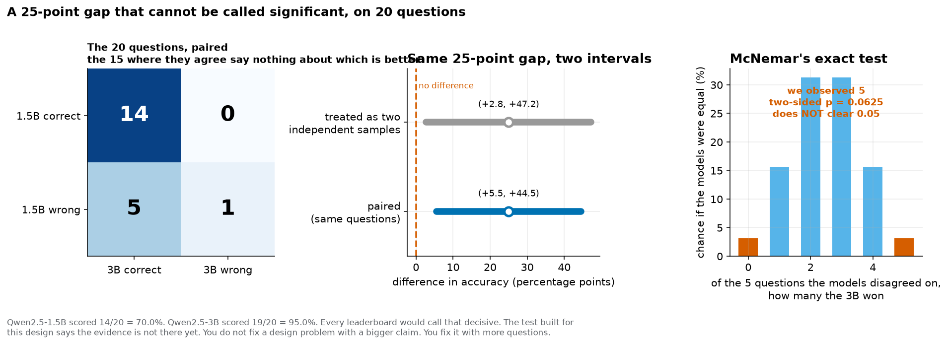
What a comparison looks like when it is reported honestly. The two-by-two table, both intervals
for the same 25 percentage point gap, and the exact test that disagrees with both of them.
Computed by lab/we7_paired_comparison.py from lab/out/we7_paired.json, on 20 questions with
rotation-debiased scoring. Your capstone’s comparison figure should contain the same three
things.
3.3 Python
Load the real paired results and rebuild the interval from the per-question score vectors, which is what your own notebook will do with your own data.
# Open the paired comparison the Chapter 13 experiment wrote.
paired_file = open("lab/out/we7_paired.json")
paired_results = json.load(paired_file)
paired_file.close()

# Name the two models explicitly. Never rely on dictionary ordering to tell them apart.
smaller_model_name = "Qwen/Qwen2.5-1.5B-Instruct"
larger_model_name = "Qwen/Qwen2.5-3B-Instruct"

# Each of these is a list of 20 numbers: 1.0 for correct, 0.0 for wrong, question by question.
smaller_model_scores = numpy.array(paired_results["per_question"][smaller_model_name])
larger_model_scores = numpy.array(paired_results["per_question"][larger_model_name])

# The pairing happens on this line. Subtract question by question, not average by average.
per_question_difference = larger_model_scores - smaller_model_scores

number_of_questions = len(per_question_difference)
mean_difference = per_question_difference.mean()

# ddof=1 divides by n minus 1, which is the n-1 in Formula 4.
difference_sd = per_question_difference.std(ddof=1)

paired_standard_error = difference_sd / math.sqrt(number_of_questions)
paired_low = mean_difference - z_for_95_percent * paired_standard_error
paired_high = mean_difference + z_for_95_percent * paired_standard_error

print("questions              :", number_of_questions)
print("mean paired difference :", mean_difference)
print("sd of the differences  :", difference_sd)
print("paired standard error  :", paired_standard_error)
print("95 per cent interval, in percentage points:", paired_low * 100, "to", paired_high * 100)
print("interval recorded in the file             :", paired_results["paired"]["ci"])
print("unpaired standard error, for comparison   :", paired_results["unpaired"]["se"])
print("the unpaired interval is this much wider  :", paired_results["width_ratio"])
print("McNemar exact two-sided p                 :", paired_results["mcnemar_exact_p"])
questions : 20
mean paired difference : 0.25
sd of the differences : 0.4442616583193193
paired standard error : 0.09933992677987828
95 per cent interval, in percentage points: 5.529374351143856 to 44.47062564885614
interval recorded in the file : [0.055293743511438564, 0.44470625648856144]
unpaired standard error, for comparison : 0.11346805717910219
the unpaired interval is this much wider : 1.1422200605254083
McNemar exact two-sided p : 0.0625The standard deviation, 0.4442616583193193, is the number Step 6 of the worked example produced
by hand, carried to more decimal places, which is the point of doing it by hand once. The interval agrees with the one
recorded in the file to every digit shown.
The last three lines are the ones to carry into your report. The unpaired standard error is 0.11346805717910219 against the paired 0.09933992677987828, so the unpaired interval is 1.14 times wider on exactly the same data. That is a real gain and it is a modest one. Pairing pays off most when the two systems agree often and the disagreements are balanced, and you should not oversell it in your report.
Then the last line, 0.0625, disagrees with both intervals. Two reasonable analyses of one
comparison point in opposite directions, and the one built for the design is the one to believe.
A capstone that reports this tension explicitly earns more interpretation points than one that
quietly reports whichever analysis it liked best.
Try it 2: a paired comparison by hand
You run two prompt formats on the same 10 questions. Format A gets questions 1, 2, 4, 5, 7 and 9 right. Format B gets questions 1, 2, 3, 4, 5, 7, 8 and 9 right. These scores are made up for practice, and they are kept small so that you can do every step on a phone calculator.
Write out the ten differences , defined as B’s score minus A’s score.
Build the two-by-two table and say how many discordant pairs there are.
Compute , then , then the paired standard error, then the 95 per cent interval. Show every step.
Compute McNemar’s exact two-sided p-value for these discordant pairs and say what you conclude.
4. What the run cost
4.1 Intuition
Every week of this course ended with the same fourth question: what did that cost? The capstone is where you answer it for your own work, and it is worth 30 of the 150 points on your final submission.
There is a reason this is graded rather than suggested, and it is the thesis of the whole course. A model small enough to be cheap to run is also a model cheap enough for a public university to put on every student’s laptop. Those are not two separate facts. They are one fact seen twice, and the course can measure both sides of it in the same units, in the same lab, on the same afternoon.
The measurement side is concrete. On the machine this book was written on, an NVIDIA RTX 3500 Ada
laptop GPU with an enforced 55 watt power limit, Qwen2.5-0.5B spent 0.767 joules of
electricity for every token it wrote, Qwen2.5-1.5B spent 1.133 joules, and Qwen2.5-3B spent
1.941 joules. The 3B costs 2.53 times the energy per token of the 0.5B. Those are
measured numbers from lab/out/theme_s_energy.json, sampled from the GPU’s own power meter at
about 50 readings a second while the model was generating.
The access side is the same numbers in different clothing. At half precision the 0.5B needs
0.99 gigabytes of memory, the 1.5B needs 3.09 gigabytes, and the 3B needs 6.17
gigabytes. Those three are measured too, from lab/out/lab4_size_ladder.json, and Formula 7
below rebuilds the first of them from the parameter count. A student with a 4 gigabyte laptop graphics card can run the first two and cannot
run the third. That line is not a metaphor. It is a threshold, it is in gigabytes, and a student
is on one side of it or the other.
Your resource-cost accounting has to put both sides in your report, for your own project, with the limits of the measurement stated in the same paragraph as the measurement.
4.2 The mathematics
Three formulas, and none of them is harder than multiplying and dividing.
Formula 5: energy per token
In words. Multiply the average power the machine was drawing by how many seconds it ran. That gives the total energy. Divide by how many tokens came out. That gives the energy per token.
The formula.
The symbols.
| Symbol | How to say it out loud | What it means |
|---|---|---|
| “E sub token” | the energy spent producing one token, in joules | |
| “E” | the letter chosen for energy | |
| the subscript “token” | “sub token” | a label saying which energy this is; it is not a multiplication |
| “P bar” | the average power drawn during the run, in watts. The bar means “the average of”. | |
| “t” | how long the run took, in seconds | |
| “m” | how many tokens the model produced | |
| “times” | multiply | |
| the fraction bar | “divided by” | divide the whole top by the bottom; do the multiplication on top first |
Out loud. “The energy per token is the average power times the number of seconds, all divided by the number of tokens.”
Worked, with the real measurement of Qwen2.5-1.5B. These numbers are from
lab/out/theme_s_energy.json and were measured, not invented.
Step 1, write down the three measured quantities. Average board power watts. Time seconds. Tokens produced .
Step 2, multiply power by time to get total energy in joules. joules
Step 3, divide by the token count. joules per token
Check it. A watt is defined as one joule per second, so watts times seconds gives joules and the units work out. If your answer is enormous, in the thousands, you probably used milliwatts; divide by 1,000. If it is tiny, you may have used minutes where the formula wants seconds. And the answer should be believable against the idle draw: this GPU sits at 13.834 watts doing nothing, and , so a model averaging 27.4 watts is drawing about twice idle, which is what a small model on a laptop GPU looks like.
Formula 6: turning joules into watt-hours for your whole project
In words. Multiply the energy per token by how many tokens your whole project generated, then divide by 3,600, because there are 3,600 seconds in an hour.
The formula.
The symbols.
| Symbol | How to say it out loud | What it means |
|---|---|---|
| “W” | the energy of the whole project, in watt-hours | |
| “E sub token” | the energy per token, in joules, from Formula 5 | |
| the subscript “token” | “sub token” | a label saying which energy this is; it is not a multiplication |
| “capital M” | the total tokens your whole project generated, across every run. Capital and small are two different quantities here, which is why the case matters. | |
| 3600 | “three thousand six hundred” | the number of seconds in an hour, which is what converts joules to watt-hours |
| “times” | multiply | |
| the fraction bar | “divided by” | divide the whole top by 3,600, so finish the multiplication on top first |
Out loud. “The watt-hours are the joules per token times the total tokens, all divided by three thousand six hundred.”
Worked, part measured and part planned. Your capstone runs 60 questions, four rotations each, on Qwen2.5-1.5B, plus pilot runs and re-runs, and you count 60,000 generated tokens in total. The per-token figure is the measured one above.
Step 1, multiply. joules
Step 2, divide by 3,600. watt-hours
Check it. Sanity-check it against something you know. A 60 watt light bulb left on for one hour uses 60 watt-hours, so twenty minutes of it is watt-hours. Your whole project came to 18.889 watt-hours, and , so your entire capstone project cost less electricity than leaving one old light bulb on for twenty minutes. That is a true and useful comparison and it belongs in your report, because it stops readers from either panicking or dismissing the number. Then say the other true thing beside it: this figure covers one laptop’s GPU, and the world runs a great many of these.
Formula 7: how much memory a model needs
In words. Multiply the number of parameters by how many bits each one is stored in, then divide by 8 to turn bits into bytes.
The formula.
The symbols.
| Symbol | How to say it out loud | What it means |
|---|---|---|
| “B” | the size of the model in bytes | |
| “capital N” | how many parameters the model has. For Qwen2.5-0.5B-Instruct this is 494,032,768. | |
| “b” | how many bits each parameter is stored in: 32 for full precision, 16 for half precision, 8 or 4 for quantized | |
| 8 | “eight” | the number of bits in one byte |
| “times” | multiply | |
| the fraction bar | “divided by” | divide the top by 8 |
Out loud. “The size in bytes is the number of parameters times the bits per parameter, all divided by eight.”
Worked, with the real parameter count of Qwen2.5-0.5B-Instruct. The count 494,032,768 is
measured, from lab/out/lab4_size_ladder.json.
The commas in a number this long are only spacers, grouping the digits in threes from the right so the eye can find the millions. They are not decimal points and they do not change the value. 494,032,768 is four hundred and ninety-four million and a bit. The Math Toolkit also writes numbers this size in scientific notation, which is the shorter way to say the same thing.
Step 1, write down the two numbers. and , because half precision stores each parameter in 16 bits.
Step 2, multiply. bits
Step 3, divide by 8. bytes
Step 4, turn bytes into gigabytes by dividing by one billion. gigabytes
Check it. At 16 bits each parameter takes exactly 2 bytes, so the answer should be almost exactly twice the parameter count with the decimal point moved: 494 million parameters gives 988 million bytes, which is 0.99 gigabytes. If your answer came out eight times too big you forgot to divide by 8. If it came out at 0.494 gigabytes you used 8 bits instead of 16.
4.3 Python
Build the resource-cost accounting for a project, starting from the measured per-token rate.
# Open the energy measurements this course made on its own hardware.
energy_file = open("lab/out/theme_s_energy.json")
energy_results = json.load(energy_file)
energy_file.close()

# Pick the model your capstone will actually use. Change this one line to change the model.
chosen_model_name = "Qwen/Qwen2.5-1.5B-Instruct"
chosen_model_energy = energy_results[chosen_model_name]

# The three measured quantities that Formula 5 needs.
mean_watts = chosen_model_energy["mean_w"]
seconds_of_generation = chosen_model_energy["seconds"]
tokens_generated = chosen_model_energy["tokens"]

# Formula 5, in two steps so you can see both halves.
total_joules = mean_watts * seconds_of_generation
joules_per_token = total_joules / tokens_generated

print("mean board power, watts   :", mean_watts)
print("seconds of generation     :", seconds_of_generation)
print("tokens generated          :", tokens_generated)
print("total energy, joules      :", total_joules)
print("energy per token, joules  :", joules_per_token)
print("value recorded in the file:", chosen_model_energy["j_per_token"])

# Formula 6. Count this number in your own notebook. Do not guess it.
tokens_my_project_will_generate = 60000
project_joules = tokens_my_project_will_generate * joules_per_token
project_watt_hours = project_joules / 3600

print()
print("tokens my project will generate:", tokens_my_project_will_generate)
print("estimated project energy, joules     :", project_joules)
print("estimated project energy, watt-hours :", project_watt_hours)
mean board power, watts : 27.408872950819674
seconds of generation : 4.961946249008179
tokens generated : 120
total energy, joules : 136.0013543278614
energy per token, joules : 1.133344619398845
value recorded in the file: 1.133344619398845
tokens my project will generate: 60000
estimated project energy, joules : 68000.6771639307
estimated project energy, watt-hours : 18.88907698998075The line to notice is the sixth one. The value your code computed from power and time,
1.133344619398845, is identical to the value recorded in the file. That is the check that your
arithmetic reproduces the lab’s, and your capstone notebook should contain a check of the same
kind somewhere.
Compare these printed values with the by-hand ones in Formulas 5 and 6 and you will find small differences, and the differences are worth understanding rather than ignoring. By hand the total came to 136.001348 joules; here it prints as 136.0013543278614. By hand the project energy came to 68,000.70 joules; here it prints as 68000.6771639307. The by-hand figures carry the rounding of the inputs you were given, because the worked example started from a power of 27.408873 watts rather than 27.408872950819674. Python started from the full number and never rounded. Both agree to six significant figures, which is far tighter than anything your report will claim, and the lesson is the one from Section 1.3: let the machine carry the digits and round once, at the end.
The last line, 18.88907698998075 watt-hours, goes in your report rounded to 18.889 watt-hours and labelled as an estimate computed from a measured rate.
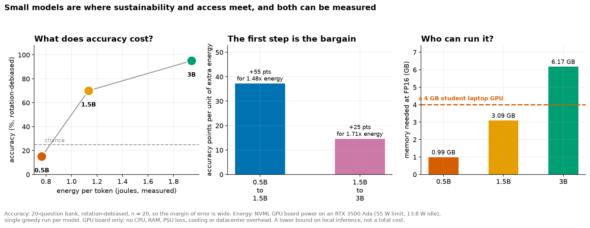
The shape a resource-cost figure should have. Accuracy from lab4_size_ladder.json, energy from
theme_s_energy.json, memory computed as two bytes per parameter. The accuracy rests on 20
questions, so its margin of error is wide; the energy rests on one greedy run per model and
covers GPU board power only. Both caveats are printed under the figure rather than left out of
it.
Try it 3: a resource-cost accounting
Your capstone uses Qwen2.5-0.5B-Instruct at half precision. Your notebook counts 24,000 generated
tokens across all your runs. That token count is made up for practice; in your own project
you will count it. The rate of 0.767069 joules per token, the above-idle rate of 0.267794 joules
per token, and the parameter count of 494,032,768 are all measured, from
lab/out/theme_s_energy.json and lab/out/lab4_size_ladder.json.
Compute the total energy in joules.
Convert it to watt-hours.
Compute the memory the model needs at half precision, in gigabytes.
Compute the energy again using the “above idle” rate of 0.267794 joules per token, and say in one sentence which of the two numbers belongs in your report.
4.4 Worked example 15.2: one project, all three slots
This is the whole capstone reduced to arithmetic. The counts are made up, so that you can check
every step; the per-token energy rate and the parameter count are measured, from
lab/out/theme_s_energy.json and lab/out/lab4_size_ladder.json.
The setup. A bank of 60 questions. One model, Qwen2.5-1.5B-Instruct. The model answered 39 correctly. Across the pilot run, the full run and two re-runs, the notebook counted 60,000 generated tokens.
Slot one, the estimate. Formula 1.
per cent.
Slot two, the interval. Formula 2, step by step.
So the 95 per cent interval is , which is 52.9 per cent to 77.1 per cent.
Slot three, the cost. Formula 6 for the energy, using the measured rate of 1.133345 joules per token.
joules watt-hours
Then Formula 7 for the memory, using the measured parameter count 1,543,714,304 at 16 bits.
bits bytes gigabytes
The three sentences that go in the report.
Qwen2.5-1.5B-Instruct answered 39 of 60 questions correctly, which is 65.0 per cent, with a 95 per cent Wald interval of 52.9 per cent to 77.1 per cent. The project generated 60,000 tokens in total, an estimated 18.889 watt-hours at the measured rate of 1.133345 joules per token on an RTX 3500 Ada laptop GPU, a figure that covers GPU board power only and excludes CPU, RAM, power-supply losses and cooling. The model needs 3.087 gigabytes at half precision, so it fits on a 4 gigabyte student laptop GPU while the 3B model, at 6.172 gigabytes, does not.
Check the whole thing. Three tests. The estimate sits inside its own interval, which it must. The interval is symmetric around the estimate, because a Wald interval always is: and , and those agree. And the memory figure is about twice the parameter count with the decimal point moved, because 16 bits is 2 bytes: 1.54 billion parameters gives 3.09 gigabytes.
5. Planning the work: five milestones and a run-time budget
5.1 Intuition
The most common way a capstone fails is not a wrong analysis. It is a student who starts running things in Week 14 and discovers that the run takes longer than the time remaining, or that the code crashes on question 51, or that the question was never answerable in the first place.
Every one of those is preventable, and the prevention is dull: find out early. The milestones exist to force the finding-out. Each one is small, each is worth 10 points, and each is designed to fail cheaply.
Milestone 2 is the important one and it is the one students most want to skip. It asks for a pilot run: ten questions, the whole procedure, end to end, producing one number. Ten questions is far too few to conclude anything, and concluding something is not the point. The point is that a pilot run finds the broken things while they are still cheap to fix.
The other thing to find out early is how long your real run will take, and that is arithmetic rather than guesswork. You can measure the cost of one trip through the model and multiply.
5.2 The mathematics
Formula 8: how long your run will take
In words. Work out how many trips through the model your run needs by multiplying the number of questions by the number of rotations by the number of models. Then multiply that by how long one trip takes.
The formula.
The symbols.
| Symbol | How to say it out loud | What it means |
|---|---|---|
| “capital T” | the estimated total run time, in seconds | |
| “q” | how many questions are in your bank | |
| “r” | how many rotations you score each question with. It is 1 if you use no rotation and 4 for the four-way rotation of this course. | |
| “k” | how many models you are running | |
| “s” | how many seconds one forward pass takes on your machine | |
| “times” | multiply | |
| the brackets | “bracket, bracket close” | do what is inside the brackets first |
Out loud. “The run time is q times r times k, all multiplied by the seconds one pass takes.”
Worked, with the real timings of Qwen2.5-0.5B-Instruct. The lab measured 6.381844 seconds for
100 forward passes, from lab/out/lab4_size_ladder.json. That 100 is itself arithmetic: the lab
scored 20 questions and made 5 passes at each one, one plain pass plus four rotations, so
. Your bank has 60 questions, you use four-way rotation, and you run one
model.
Step 1, find the seconds per pass from the measurement. seconds per pass
Step 2, count the passes your run needs. passes
Step 3, multiply. seconds
Now do it again for the 3B model, whose measurement was 20.621242 seconds for 100 passes. seconds per pass seconds
Check it. The bigger model must be slower per pass, and 0.206 seconds is more than 0.064 seconds, so the two agree with each other. If your estimate for the big model came out faster, you divided by the wrong pass count. And scale the answer up to feel whether it is plausible: a 1,000-question bank on the 3B with four rotations is seconds, which is under 14 minutes, so a big bank is not out of reach on a single afternoon.
The number that surprises students is how small is. A 60-question capstone run finishes in under a minute of actual computing. The run is never the slow part. Writing the questions is the slow part, and so is loading the model, which took 18.8 seconds for the 3B on the lab machine, and so is the first run of the day while the software compiles its kernels. Budget your weeks around writing and debugging, not around waiting.
5.3 Python
Estimate your own run time from the lab’s measured timings, for each of the three models.
# Open the size-ladder run, which recorded how long each model took.
ladder_file = open("lab/out/lab4_size_ladder.json")
ladder_results = json.load(ladder_file)
ladder_file.close()

# The three things you decide. Change these to match your own plan.
questions_in_my_bank = 60
rotations_per_question = 4
models_i_will_run = 1

# Formula 8, first bracket: the number of forward passes.
forward_passes_needed = questions_in_my_bank * rotations_per_question * models_i_will_run
print("forward passes my run needs:", forward_passes_needed)
print()
print("model                       seconds per pass    estimated run seconds")

# Walk the three models one at a time with an explicit for loop.
for model_name in ladder_results:
    one_model = ladder_results[model_name]
    # The lab scored 20 questions with 5 passes each, so 100 passes in total.
    measured_seconds = one_model["infer_s"]
    measured_passes = one_model["n"] * 5
    seconds_per_pass = measured_seconds / measured_passes
    estimated_seconds = forward_passes_needed * seconds_per_pass
    print(model_name, round(seconds_per_pass, 6), round(estimated_seconds, 1))
forward passes my run needs: 240
model seconds per pass estimated run seconds
Qwen/Qwen2.5-0.5B-Instruct 0.063818 15.3
Qwen/Qwen2.5-1.5B-Instruct 0.0806 19.3
Qwen/Qwen2.5-3B-Instruct 0.206212 49.5Three sentences about that table.
The seconds per pass climbs with model size, from 0.063818 seconds on the 0.5B to 0.206212 seconds on the 3B. That is , so a factor of about 3.2, for a model with times the parameters. The estimated run times, 15.3 to 49.5 seconds, are all short enough that the size of your bank is limited by how many questions you can write, not by how long the machine takes. And these timings were measured on the machine described in the lab notebook, so your own machine will differ, which is exactly why Milestone 2 asks you to run a pilot and time it yourself rather than trusting this table.
5.4 The milestone schedule
Five checkpoints, 10 points each, 50 points in total. Each is small on purpose. Submitting nothing on a milestone costs 10 points; submitting something incomplete and honest costs very little.
| # | Due | What you submit | 10 points are for | Feedback you get back |
|---|---|---|---|---|
| M1 | Week 9 | One page: your question in one sentence, the model, the bank you will build, the scoring procedure, the sample size, and the margin of error you computed from Formula 3. This is your preregistration. | being specific enough to execute, not for being right | a yes, or one concrete change to make |
| M2 | Week 11 | A pilot run: 10 questions, the full procedure, end to end, one number printed by code that runs on a fresh kernel. | the code running, not the number it prints | where it will break at full size |
| M3 | Week 12 | The full run, with the headline number and its 95 per cent interval, computed in your own notebook. | an interval present and correct | whether the interval method fits your design |
| M4 | Week 13 | Your comparison done as a paired analysis, or one paragraph saying why your design is not paired. | matching the analysis to the design | a check on the pairing |
| M5 | Week 14 | The resource-cost table, plus the self-check further down this chapter, completed and signed. | the table and the signed checklist | the last chance to fix something before grading |
| Final | Week 15 | The three-minute talk and the final report. | graded on the 150-point rubric in Section 6 | your grade, with the rubric filled in row by row |
6. How this is graded, as arithmetic
6.1 Intuition
A rubric that is published in advance and computed in public is not a formality. It is the same idea as preregistration, applied to grading: the standard is fixed before the work is seen, so the grade is a measurement rather than an impression.
Here is the shape. The capstone is 200 points. The five milestones are 10 points each, so points, described above. That leaves points for your final submission, the report and the talk together, graded on four criteria.
The weights say what the course values, and they are not evenly spread:
| Criterion | Points | Share of the 150 |
|---|---|---|
| Correct method | 60 | 40 per cent |
| Honest interpretation | 45 | 30 per cent |
| Resource-cost accounting | 30 | 20 per cent |
| Communication | 15 | 10 per cent |
| Total | 150 | 100 per cent |
Each share in the last column is the points divided by 150, turned into a percentage by multiplying by 100. For the first row, , and per cent. For the others, , and .
Read those weights as a sentence. Doing the right thing with the data is worth the most. Saying truthfully what it does and does not show is worth the next most, and it is worth twice what the writing quality is worth. Accounting for what it cost is worth half again as much as the writing. And the writing still matters, because a result nobody can follow has not been reported.
6.2 The mathematics
Adding the rows up is a weighted sum, and it is the only place in this chapter where sigma notation appears.
Formula 9: your capstone score
In words. For each criterion, multiply the points it is worth by the fraction of them you earned. Add up those products. That total is your score on the final submission.
The formula.
The symbols.
| Symbol | How to say it out loud | What it means |
|---|---|---|
| “score” | the points you earned on the final submission, out of 150 | |
| “sigma”, or “the sum of” | add up everything that follows, once for each value of the counter | |
| “eye” | the counter. is the first criterion, the second. | |
| underneath the sigma | “i equals one” | start the counter at 1 |
| on top of the sigma | “k” | stop the counter at . Here , because there are four criteria. |
| “w sub i” | the points criterion number is worth: 60, 45, 30 or 15 | |
| “s sub i” | the fraction of criterion you earned, a number between 0 and 1 | |
| “w sub i s sub i” | two symbols written side by side means multiply them |
If sigma notation is still uncomfortable, the Math Toolkit builds it from scratch, starting from “add these up”. The formula above is nothing more than written shorter.
Out loud. “The score is the sum, for each criterion from the first to the fourth, of that criterion’s points times the fraction of them you earned.”
Worked, with made-up scores for an imagined report. A report that does the method well, is a bit hedgy in its interpretation, nails the cost accounting, and is hard to read.
Step 1, list the four criteria with their points and fractions earned.
| Criterion | ||||
|---|---|---|---|---|
| 1 | correct method | 60 | 0.90 | |
| 2 | honest interpretation | 45 | 0.80 | |
| 3 | resource accounting | 30 | 1.00 | |
| 4 | communication | 15 | 0.70 |
Step 2, add the last column.
Step 3, turn it into a percentage of the final submission. , so per cent.
Step 4, add the milestone points. Suppose all five were submitted on time and complete, so 50 out of 50. out of 200. , so per cent of the capstone.
Check it. Every must be between 0 and ; a product larger than the points available means a fraction above 1 was entered. And the total must be at most 150; if it is not, add the column again.
6.3 The four criteria, line by line
Each criterion breaks into items. This is the sheet your work is marked against.
Correct method, 60 points.
| Item | Points | What earns them |
|---|---|---|
| M1 | 10 | the question names a measurable quantity, a model, a procedure and a sample size |
| M2 | 15 | the procedure is fixed in advance and described so a classmate could repeat it exactly |
| M3 | 15 | the comparison is paired when the design is paired, and unpaired when it is not |
| M4 | 20 | the notebook runs top to bottom on a fresh kernel and produces every number in the report |
Honest interpretation, 45 points.
| Item | Points | What earns them |
|---|---|---|
| H1 | 20 | every headline number is reported with an interval. A bare accuracy scores zero here. |
| H2 | 10 | the interval is computed by a method that fits the design, and the method is named |
| H3 | 10 | the conclusion does not claim more than the interval supports |
| H4 | 5 | limitations are named in the report, not left for the reader to notice |
Resource-cost accounting, 30 points.
| Item | Points | What earns them |
|---|---|---|
| R1 | 10 | energy per token measured, or [not measured] with a stated reason, and the method named |
| R2 | 10 | total energy for the whole project, in joules and watt-hours, labelled as measured or estimated |
| R3 | 5 | memory footprint in gigabytes, and one sentence on who can and cannot run this model |
| R4 | 5 | the limits of the measurement stated in the same section as the measurement |
Communication, 15 points.
| Item | Points | What earns them |
|---|---|---|
| C1 | 5 | the report is within 1,500 to 2,500 words and readable by a classmate who did not do your project |
| C2 | 3 | every figure has a caption and alt text, and no figure uses colour as its only signal |
| C3 | 4 | the talk lands inside three minutes |
| C4 | 3 | the summary slide states the claim, the interval and the cost |
6.4 Python
Score a draft against the rubric before you hand it in. Change the fractions to your own honest estimates.
# Three parallel lists, written out in full. The four criteria stay in the same order in all
# three, so position 0 means "correct method" in every one of them.
criterion_names = ["correct method", "honest interpretation", "resource accounting", "communication"]
criterion_points = [60, 45, 30, 15]

# Your honest estimate of the fraction of each criterion your draft earns, from 0.0 to 1.0.
criterion_fraction_earned = [0.90, 0.80, 1.00, 0.70]

# Formula 9. An explicit for loop that adds one criterion at a time.
running_total = 0.0
for criterion_index in range(len(criterion_names)):
    points_available = criterion_points[criterion_index]
    fraction_earned = criterion_fraction_earned[criterion_index]
    points_earned = points_available * fraction_earned
    running_total = running_total + points_earned
    print(criterion_names[criterion_index], points_available, "x", fraction_earned, "=", points_earned)

print("final submission total, out of 150:", running_total)
print("as a percentage                   :", running_total / 150 * 100)

# Add the milestone points to get the capstone total out of 200.
milestone_points_earned = 50
capstone_total = milestone_points_earned + running_total
print("capstone total, out of 200        :", capstone_total)
print("as a percentage                   :", capstone_total / 200 * 100)
correct method 60 x 0.9 = 54.0
honest interpretation 45 x 0.8 = 36.0
resource accounting 30 x 1.0 = 30.0
communication 15 x 0.7 = 10.5
final submission total, out of 150: 130.5
as a percentage : 87.0
capstone total, out of 200 : 180.5
as a percentage : 90.25Run this once in Week 13 and once again in Week 14, and be hard on yourself both times. The useful output is not the total. It is the line with the lowest product in it, because that is the criterion where an hour of work buys you the most.
In the run above the smallest product is communication at 10.5 points. But the largest available gain is elsewhere: interpretation is at 0.80 of 45 points, so getting it to 1.00 is worth points, while getting communication from 0.70 to 1.00 is worth points. Multiply the gap by the weight, not by your feelings about the row.
6.5 Worked example 15.3: two drafts, scored
Two students submit reports on the same question. Both did the same amount of work. Here is why they receive different grades. The counts and percentages in both drafts are invented for this example; the 3B model’s measured score in this course is 95.0 per cent on 20 questions, not the 65.0 per cent these two imagined students report.
Draft A, result section, in full.
Qwen2.5-3B-Instruct answered 39 of 60 questions correctly, which is 65.0 per cent. The 95 per cent Wald interval is 52.9 per cent to 77.1 per cent, computed as . The interval is wide because 60 questions is a small bank; Formula 3 says a 10 point margin needs 97 questions. I therefore cannot distinguish this model from one whose true accuracy is 55 per cent, and I do not claim to.
Draft B, result section, in full.
Qwen2.5-3B-Instruct scored 65 per cent, showing it has a solid grasp of introductory statistics.
Draft A scores full marks on H1, H2 and H3. It reports the number, the interval, the method that produced the interval, and a conclusion that stays inside the interval. The final sentence, which declines to claim something, is the sentence that earns the most points in the paragraph.
Draft B scores zero on H1 and zero on H2, because there is no interval. It also scores zero on H3, because “a solid grasp” is a claim the data cannot support: the honest interval reaches down to 52.9 per cent, which is not far above the 25 per cent you would get by guessing on four options. That is of the 45 interpretation points gone from one sentence.
The difference between the two drafts is not effort, cleverness or writing ability. It is three extra lines of arithmetic and one sentence of restraint.
Try it 4: score a draft yourself
A draft has these features. The notebook runs end to end and produces every number. The design
was paired and the student analysed it as paired, naming the method. Every headline number has an
interval. The conclusion says “the 3B model is definitively better”, although the interval runs
from +5.5 to +44.5 percentage points and McNemar’s exact test gives . The energy
row says [not measured] with no reason given. Memory and limits are both reported. The report
is 2,100 words with captioned figures, and the talk ran 4 minutes 10 seconds.
Score each of the four criteria item by item, using the tables in Section 6.3.
Use Formula 9 to compute the total out of 150, and the percentage.
Name the one change that buys the most points.
7. The talk
7.1 Intuition
The last thing you do in this course is stand up and take three minutes to say what you found. Three minutes is short enough to be frightening and short enough to be survivable, and it is not an arbitrary number.
The limit comes out of arithmetic that you can check, and knowing that makes it easier to accept. This section meets for 150 minutes a week and seats up to 45 students. Everyone presents in Week 15. Changing speakers, plugging in a laptop and settling the room takes about 15 seconds each time. Section 7.2 does the multiplication and the answer is that three minutes fits with 3.75 minutes to spare and five minutes does not fit at all.
So the format is fixed, and here it is.
Three minutes, hard stop. A timer runs on the screen. At three minutes you stop, mid-sentence if necessary. This is worth 4 points on the rubric and it is the easiest 4 points in the course, because the only thing it requires is rehearsing once with a clock.
Three slides, no more.
| Slide | What is on it | The sentence you say |
|---|---|---|
| 1. The question | your one-sentence question, the model’s name, the size of your bank | “I asked whether ... on ... questions.” |
| 2. The method and the number | how you scored, the headline number, and the interval beside it | “I scored it this way. It got X per cent, 95 per cent interval Y to Z.” |
| 3. The cost and the caveat | the energy, the memory, and the one thing you cannot conclude | “It cost this much energy and needs this much memory, and here is what I cannot claim.” |
One question from the floor. After each talk, one person asks one question. You may not be asked the same question twice in the room, so listen to the ones before yours.
The question you should expect. Somebody will ask what your interval is. If it is already on slide 2, the answer takes four seconds and you look prepared. That is the whole reason it is on slide 2.
7.2 The mathematics
Formula 10: does the schedule fit?
In words. Add the length of one talk to the time it takes to swap speakers. Multiply by the number of talks. Compare that with the minutes the class actually has.
The formula.
The symbols.
| Symbol | How to say it out loud | What it means |
|---|---|---|
| “T sub total” | the total minutes the session needs | |
| “k” | how many talks there are, which is how many students present | |
| “t” | the length of one talk, in minutes | |
| “c” | the changeover time between talks, in minutes | |
| “t plus c” | the minutes one speaker consumes in total | |
| “times” | multiply | |
| the brackets | “bracket, bracket close” | do the addition inside before multiplying |
Out loud. “The total time is the number of talks, times the length of one talk plus the changeover.”
Worked, with the real section size. The course’s section size is 45 students, from the course specification. A changeover of 15 seconds is minutes.
Step 1, add the talk and the changeover. minutes per speaker
Step 2, multiply by the number of talks. minutes
Step 3, compare with the minutes available. minutes spare.
Now test five-minute talks, which is what students usually ask for. minutes per speaker minutes
Step 4, compare. minutes over. Five-minute talks need more than an extra full session.
Check it. The total must grow when either or grows. Halving the class to 22 or 23 students would make five-minute talks fit: minutes, which is inside 150. So the limit is a fact about the room, not about you, and if your section is smaller your instructor may extend it.
7.3 Python
Check your own schedule arithmetic, then print the three lines that go on your slides, so the slide and the notebook cannot disagree.
# Formula 10. Change these four numbers to match your own section.
talks_to_fit = 45
minutes_per_talk = 3.0
minutes_for_changeover = 0.25
minutes_available = 150.0

minutes_needed = talks_to_fit * (minutes_per_talk + minutes_for_changeover)

print("talks to fit        :", talks_to_fit)
print("minutes per talk    :", minutes_per_talk)
print("changeover per talk :", minutes_for_changeover)
print("minutes needed      :", minutes_needed)
print("minutes available   :", minutes_available)
print("minutes left over   :", minutes_available - minutes_needed)

# Now print the slide text from your own results, so the slide cannot drift from the notebook.
# Replace every value below with a number your own code produced.
my_claim = "Qwen2.5-3B-Instruct scored higher than Qwen2.5-1.5B-Instruct on my 20-question bank."
my_estimate_points = 25.0
my_interval_low = 5.5
my_interval_high = 44.5
my_energy_watt_hours = 18.889

print()
print("SLIDE 2, the number:")
print("  claim   :", my_claim)
print("  estimate:", my_estimate_points, "percentage points")
print("  interval:", my_interval_low, "to", my_interval_high, "percentage points")
print("SLIDE 3, the cost:")
print("  energy  :", my_energy_watt_hours, "watt-hours for the whole project")
talks to fit : 45
minutes per talk : 3.0
changeover per talk : 0.25
minutes needed : 146.25
minutes available : 150.0
minutes left over : 3.75
SLIDE 2, the number:
claim : Qwen2.5-3B-Instruct scored higher than Qwen2.5-1.5B-Instruct on my 20-question bank.
estimate: 25.0 percentage points
interval: 5.5 to 44.5 percentage points
SLIDE 3, the cost:
energy : 18.889 watt-hours for the whole projectThe second half of that cell looks trivial and it prevents a specific failure. Slides get made on Sunday night and numbers get edited on Monday, and the slide keeps the old number. Printing your slide text from the same notebook that produced the numbers means the two cannot drift apart. Copy the printed lines onto the slide rather than typing them in.
The numbers in that example are the real paired comparison from lab/out/we7_paired.json, on the
20-question bank of Chapter 13, and the estimated project energy from Section 4. They are placed
there so you can see the shape. Replace all five with your own.
The checklist, to run against your own draft
Go through this before you submit, with the draft open. Every line maps to a rubric item, and the item number is printed beside it so you can see what each answer is worth.
The question and the method
My question names a model, by its full name including the size. (M1)
My question names a measurable quantity, and I could say what units it is in. (M1)
My question names the scoring procedure and the size of the bank. (M1)
My method section is detailed enough that a classmate could repeat my run without asking me anything. (M2)
Any random seed is set explicitly in the notebook. (M2)
If I changed my procedure after Milestone 1, the report says so and says why. (M2)
If both systems answered the same items, my analysis is paired, and I say so. (M3)
My notebook runs top to bottom on a fresh kernel with no errors. (M4)
Every number in my report appears in my notebook’s printed output. (M4)
The result and the honesty
Every headline number in my report has an interval beside it. Every one. (H1)
I have checked the abstract, the conclusion and every figure caption for a bare number. (H1)
I name the method that produced each interval: Wald, Wilson, bootstrap or paired. (H2)
The method I used fits my design rather than the one I found first. (H2)
My conclusion stays inside my interval. I have reread it looking for “clearly”, “proves”, “definitively” and “shows that”. (H3)
If two analyses disagree, I report both and say which one the design supports. (H3)
I have a limitations paragraph and it names my sample size as a limitation. (H4)
The cost
I report energy per token, measured, or
[not measured]with a stated reason. (R1)I report total project energy in joules and in watt-hours. (R2)
Every energy row says whether it was measured or estimated from a measured rate. (R2)
I report memory in gigabytes and say who can and cannot run this model. (R3)
The limits of my measurement are in the same section as the measurement. (R4)
The writing and the talk
The report is between 1,500 and 2,500 words. I have counted, not guessed. (C1)
Somebody who did not do my project has read it and can say what I found. (C1)
Every figure has a caption and alt text. (C2)
No figure uses colour as its only signal. (C2)
I have rehearsed the talk with a timer and it lands under three minutes. (C3)
Slide 2 shows the claim, the estimate and the interval. (C4)
The honesty policy
Every number in this report was computed by code I ran.
No number came from a chatbot, an estimate, or a memory of something I read.
Any invented number in a worked example is labelled as invented.
The AI-use disclosure box is filled in: which tool, what I asked, what I did with the answer.
Milestone 5 asks you to submit this checklist completed and signed. Ticking a box you have not checked is the one thing on this list that is dishonest rather than incomplete.
Common mistakes
Reporting a bare accuracy. The single most expensive mistake in the capstone, worth 30 of 150 points. How to spot it: search your draft for the per cent sign and look at every hit. If the number next to it has no interval within one sentence, fix it.
Choosing paired or unpaired after seeing which gives the nicer answer. How to spot it: if you cannot point at the sentence in your Milestone 1 submission where you named the analysis, you chose it after the fact.
Rounding partway through. Rounding a standard error from 0.09682458365518543 to 0.1 before multiplying by 1.96 moves the interval by about 0.6 percentage points for no reason. How to spot it: your number differs from the checked value in the second decimal place. Carry full precision and round once, at the end.
Confusing per cent with percentage points. A model going from 70.0 per cent to 95.0 per cent gained 25.0 percentage points, not 25 per cent. As a per cent it rose by 35.7 per cent of its old value. Work left to right: , then , which rounds to 35.7. How to spot it: a difference between two percentages is always in percentage points.
Quoting a number you did not compute. Reading “a ChatGPT query uses about 3 watt-hours” somewhere and putting it in your table. How to spot it: for every number in your report, name the line of your notebook that produced it. If you cannot, it does not belong in a row with ones you did compute.
Treating the pilot run as a result. Ten questions cannot support a claim. At and the margin of error is 31.0 percentage points: , then , then , then , then . How to spot it: your result section cites a number from Milestone 2.
Blaming the model for the scorer. Chapter 13’s naive procedure reported 25.0 per cent when it was measuring the model’s preference for the letter A, chosen on 16 of 20 questions, both recorded in
lab/out/we6b_eval_debiased.json. How to spot it: print the spread of your model’s chosen letters. If one letter dominates, your scorer is the thing you are measuring.Leaving the energy row blank rather than writing
[not measured]. A blank cell reads as an oversight and scores zero.[not measured], with one sentence of reason, scores full marks on R1. How to spot it: look for empty cells in your cost table.Letting the talk run long. Four minutes ten seconds costs 4 points on C3 and it costs the next speaker their time. How to spot it: rehearse once with a clock. That is the whole fix.
Starting the run in Week 14. How to spot it: you have not submitted Milestones 1 to 4. Every milestone you skip removes a checkpoint that would have caught the problem while it was still small.
What to remember
A capstone result is three things, an estimate, an interval and a cost, and a report with only the first one is not finished. The question you write in Week 9 decides everything that follows, so make it name a model, a quantity, a procedure and a sample size. Precision costs questions at four times the rate you expect, so plan the bank size with Formula 3 before you write a single question. When two systems answer the same items, the analysis is paired, and you choose that because of the design rather than because of the answer. Write down what you cannot conclude, in your own words, because that sentence is worth more points than any other sentence in the report.
Practice problems
Two notes before you start.
Where the numbers come from. A problem that names a file in lab/out/ is using a measured
number, and your answer should reproduce it. Every other number in this set is made up for
practice and is kept small so you can work it on a phone calculator.
Where the answers are. Worked solutions to the odd-numbered problems are in the answers appendix, the same as every other chapter. Two of them, problems 3 and 15, build on an even-numbered problem whose answer is not published, so each of those solutions restates the earlier result it needs before using it. You can work them without having done the even-numbered problem first.
Every method these problems use is also worked in full earlier in this chapter, and the standing computations behind them are worked again in the appendix under Chapter 12 for the interval, Chapter 13 for the paired comparison, and Chapter 7 for the bytes-per-weight arithmetic. Check your work against those.
Warm-up: can you do the arithmetic?
1. A model answers 27 of 45 questions correctly. Compute as a decimal and as a percentage.
2. For and , compute , then divide by , then take the square root. Show each step.
3. Using your answer to problem 2, compute the margin of error and write the 95 per cent interval as two percentages.
4. Using Formula 3 with , how many questions are needed for a margin of error of 8 percentage points? Round up to a whole question.
5. A GPU draws an average of 24.5 watts for 6.2 seconds and produces 140 tokens. Compute the total joules and the joules per token.
6. Convert 42,000 joules into watt-hours.
7. A model has 1,543,714,304 parameters stored at 16 bits each. That count is the measured
one for Qwen2.5-1.5B-Instruct, from lab/out/lab4_size_ladder.json. Compute its size in bytes
and in gigabytes.
8. A rubric criterion is worth 45 points and you earn 0.6 of it. How many points is that?
Practice: can you apply it?
9. Your bank has 100 questions and the model gets 71 right. Report the result the way the rubric requires: the headline number, the interval, and a one-sentence conclusion that stays inside the interval.
10. You want a margin of error of 5 percentage points and you expect the model to score around 0.8. Use Formula 3 with and again with . Explain in two sentences why the second answer is larger and why you should use it when planning.
11. Two models answer the same 12 questions. Model A is right on questions 1, 3, 4, 6, 7, 9 and 11. Model B is right on questions 1, 2, 3, 4, 6, 7, 9, 10 and 11. Build the two-by-two table and say how many discordant pairs there are.
12. For the data in problem 11, compute , , the paired standard error, and the 95 per cent interval. Show every step.
13. For the data in problem 11, compute McNemar’s exact two-sided p-value and say what you conclude.
14. Your project generates 35,000 tokens on Qwen2.5-3B-Instruct. Using the measured rate of
1.940526 joules per token from lab/out/theme_s_energy.json, compute the project energy in
joules and in watt-hours.
15. Compute the same project energy using the measured above-idle rate of 1.051711 joules per
token, also from lab/out/theme_s_energy.json. Write one sentence explaining what the difference between the two answers represents.
16. Your bank has 80 questions, you use four-way rotation, and you run two models. Using the
measured seconds per pass for the 1.5B model, 0.080600 seconds, from
lab/out/lab4_size_ladder.json, estimate the total run time in seconds and in minutes.
17. A draft scores 0.85 on correct method, 0.20 on honest interpretation, 0.90 on resource accounting and 1.00 on communication. Use Formula 9 to compute the total out of 150 and the percentage.
18. The 0.20 on interpretation in problem 17 came from scoring zero on H1 and zero on H2, because no interval appeared anywhere in the report. What does the total become if both items are fixed to full marks? Express the gain in points and in percentage points of the final submission.
Stretch: can you reason with it?
19. A classmate says “my interval is so wide that my project failed”. Write a three-sentence reply that explains why a wide interval honestly reported scores better on this rubric than a narrow one dishonestly produced, and name the rubric items involved.
20. In Chapter 13 the unpaired standard error was 0.11346805717910219 and the paired was
0.09933992677987828, a width ratio of 1.14, all three recorded in lab/out/we7_paired.json. Explain, in your own words and without formulas, why
the gain was modest here and describe a situation in which pairing would help far more.
21. The paired interval for the 1.5B against the 3B was percentage points,
which excludes zero, while McNemar’s exact test gave , which does not clear 0.05.
Both come from lab/out/we7_paired.json. Both
analyses are defensible. Write the paragraph you would put in a capstone report that reports both
honestly, in under 120 words.
22. Chapter 10 measured that bge-small-en-v1.5 retrieved the correct section 6 times out of
6 with a mean confidence gap of 0.055, while all-MiniLM-L6-v2 retrieved it 3 times out of 6
with a larger mean gap of 0.058. All four numbers are in lab/out/lab2_rag_v3.json. Explain why this means a confidence gap cannot be compared
across two different systems, and say what this implies for any capstone that compares two
retrieval setups.
23. Design a capstone question of your own on any topic in this course. Write it in one sentence. Then write the four things a grader would check it for under item M1, and show that your question contains all four. Finally compute, using Formula 2, the margin of error your design would carry.
24. Using the measured energy figures of 0.767069, 1.133345 and 1.940526 joules per token,
from lab/out/theme_s_energy.json, and the measured rotation-debiased accuracies of 15.0, 70.0
and 95.0 per cent, from lab/out/lab4_size_ladder.json, compute the accuracy
points gained per joule per token for the step from the 0.5B to the 1.5B, and for the step from
the 1.5B to the 3B. Then write two sentences on what that comparison says about which model a
public university with a limited budget should deploy, and one sentence on what the
bank size means for how much weight to put on your answer.