What you need before this chapter
This chapter needs five things. Four of them are pieces of notation, and every one of them has a page in the Math Toolkit that starts from nothing.
| You need | Where it is taught from zero |
|---|---|
| A letter standing for a number | Toolkit 1 |
| Subscripts, so that and mean different things | Toolkit 2 |
| The fraction bar, which means divide | Toolkit 4 |
| Exponents, and the number | Toolkit 5 and Toolkit 7 |
| The sign, which means “add these up” | Toolkit 10 |
Two more arrive inside this chapter, and this chapter teaches both of them from the beginning rather than assuming them:
| Arriving here | Also written out in the Toolkit |
|---|---|
| Logarithms, at the level of “the log tells you the exponent” | Toolkit 8 |
| Bits, and powers of two | Toolkit 18 |
The fifth thing is Chapter 4. Chapter 4 built softmax, the procedure that turns the model’s raw scores into probabilities. This chapter changes one step of that procedure and then measures what changed. If softmax is not yet solid, read Chapter 4 again before this one. Most people need two passes at Chapter 4. That is what that chapter is like, and it is not a sign you are behind.
You do not need calculus. You do not need to have programmed before. Every piece of arithmetic in this chapter is small enough to check on a phone calculator, and this chapter shows every step.
The setup code
Run this once, at the top of your session, before anything else on this page.
# Cell 1. The imports for this chapter.
# House rule, borrowed from UC Berkeley's Data Science Modules: every import lives in the
# first cell, one per line, each with a comment saying what it is for. No import appears
# further down the page. Read this one cell and you know everything the code depends on.

import os                                      # lets Python read and change settings on your computer
os.environ["HF_HOME"] = r"C:\math3219\models"  # the folder where downloaded models are kept
                                               # this line MUST come before the two transformers lines

import json                                    # reads the lab's saved .json files, which is where this book's numbers live
import math                                    # gives us the number e, the exponential, and log base 2
import random                                  # draws random numbers between 0 and 1, which is what sampling needs
import torch                                   # the arithmetic library the language models are built on
import matplotlib.pyplot as pyplot             # draws every chart in this book
from transformers import AutoTokenizer         # turns text into token ids, and ids back into text
from transformers import AutoModelForCausalLM  # loads a model that predicts the next token
If any of those lines fails, the installation section of the Python Reference walks through the fix. Nothing in this chapter requires a graphics card.
A slider in a writing app, on a hot afternoon in Bakersfield
It is August in Kern County. The thermometer outside the student union has been a conversation topic for a week. Inside, in an air-conditioned computer lab, a student opens a writing assistant and finds a slider. One end of it says Precise. The other end says Creative. There is a small number underneath the handle, and the number says 0.7.
That slider is the subject of this chapter. The number is called the temperature, and it has nothing whatever to do with heat. Underneath the slider there is one division. Not a different model, not extra imagination, not a second opinion. One division, carried out on numbers the model has already produced, before those numbers are turned into probabilities.
The label on that slider is the most dangerous sentence in this course:
“Temperature makes the model more creative.”
That sentence is wrong, and this chapter is going to say exactly how it is wrong, then measure the damage it does to your understanding. Here is the short version, which will make full sense by the end of this page. Temperature divides the scores before they are exponentiated. Dividing by a number bigger than 1 squeezes the scores together, so the probabilities get flatter. Dividing by a number smaller than 1 pushes the scores apart, so the probabilities get sharper. And dividing every score by the same positive number cannot change which score is the biggest, in the same way that halving the height of every person in a room cannot change who is tallest.
So temperature cannot reorder the model’s candidates. It cannot invent a new candidate. It cannot remove one. At a setting of exactly 1 it does not do anything at all.
What it does do is measurable, and this chapter measures it three ways on a real model. The
model is Qwen2.5-0.5B-Instruct, 494,032,768 numbers, with a vocabulary of 151,936 tokens. The
prompt is The capital of France is. Here is the headline, and you will be able to reproduce
every digit of it by the end of the chapter.
At a temperature of 0.25, one single token carries 90% of the model’s probability. At a temperature of 2.0, on exactly the same scores, it takes 41,274 tokens to carry that same 90%.
One dial. One division. A word count that goes from 1 to 41,274. No creativity anywhere.
Learning objectives
By the end of this chapter you will be able to:
State what temperature does mechanically, in one sentence containing no symbols, and point to the exact step of the softmax procedure where the division happens.
Compute a temperature-adjusted probability by hand, from raw scores, showing every division, every exponential and every sum, and check your answer by adding the results to 1.
Explain why temperature cannot change the ranking of the candidates, using either the ratio between two probabilities or the power form of the temperature formula.
Measure how spread out a distribution is, using entropy in bits and the count of tokens holding 90% of the probability, and say in plain English what each of those two numbers means.
Tell the difference between greedy decoding and sampling, and rewrite the claim “temperature makes the model more creative” into a sentence that is true and testable.
This lesson at a glance
Temperature is a division that happens before the exponential. Divide every score by the same positive number , then run softmax exactly as Chapter 4 built it.
Below 1 it sharpens, above 1 it flattens, and at exactly 1 it does nothing. Dividing by 1 leaves every score where it was.
It cannot reorder the tokens. The model’s favourite at is the same token as at , and there is a one-line reason why.
The distribution-level view is the honest one. Entropy runs from 0.237 bits to 13.367 bits across the five measured settings, and the count of tokens holding 90% of the probability runs from 1 to 41,274.
The vocabulary of this chapter
Every technical word this chapter uses, defined before it is used. Read the table once now. Each term is defined again, more slowly, at the point where it first matters.
| Term | What it means, in one line |
|---|---|
| token | One item from the model’s fixed list of 151,936 pieces of text. Not a word. |
| logit | One raw score the model gives one token. Can be negative. Said “LOW-jit”. |
| softmax | The procedure that turns a whole list of logits into probabilities that add to 1. |
| distribution | A complete list of probabilities, one for every token, adding to 1. |
| temperature | A positive number you divide every logit by before running softmax. Written . |
| scaled logit | A logit after it has been divided by the temperature. |
| sharpen | Make the leading probability bigger and the rest smaller. Happens when . |
| flatten | Make the probabilities more equal. Happens when . |
| probability mass | Probability treated as a quantity that gets shared out. It totals 1. |
| bit | The unit uncertainty is measured in. One bit is one yes-or-no question’s worth. |
| logarithm base 2 | The question “two raised to what power gives this number?” Written . |
| entropy | One number, in bits, saying how spread out a distribution is. Written . |
| nine-tenths count | How many tokens, starting from the most likely, it takes to reach 90% of the probability. Written . |
| greedy decoding | Always taking the highest-probability token. No randomness at all. |
| sampling | Drawing a token at random, giving each token a chance equal to its probability. |
| seed | A number that fixes which random draws you get, so a random procedure repeats exactly. |
| argmax | “The position of the biggest one.” A function that returns a position, not a value. |
| renormalise | Divide a shortened list of numbers by their own total so it adds to 1 again. |
5.1 What the temperature dial actually does
Intuition
Think about a school prize-giving where the judges have already scored every entry. The scores are final. Nobody is going to re-judge anything. What is left is a decision about how to hand out the prize money.
One committee says: the top entry is much better than the second, so it takes almost everything. Another committee looks at the same scores and says: these entries are all quite close, so let us spread the money around. Neither committee changed a single score. Neither committee promoted the runner-up above the winner. They made the same ranking look sharp or look flat.
Temperature is the dial that picks between those two committees, and it does it with one division.
Here is the whole mechanism. In Chapter 4 you took a score, raised to it, and divided by the total. Temperature adds one step in front of all of that: divide every score by the same number first. That number is called the temperature and it is written .
Why does dividing change the shape of the answer? Because the exponential step cares about the gaps between scores, not the scores themselves. Two scores that are 4 apart produce a very lopsided result. The same two scores divided by 2 are only 2 apart, and 2 apart produces a much more even result. Dividing by a number bigger than 1 shrinks every gap. Dividing by a number smaller than 1 stretches every gap.
That gives you the three cases, and they are worth memorising now.
below 1. Every gap gets bigger. The leader pulls away. The picture sharpens.
exactly 1. Every score divided by 1 is itself. Nothing at all happens. This is plain softmax, and it is the setting most systems ship with.
above 1. Every gap shrinks. The candidates crowd together. The picture flattens.
The one thing that never happens, at any setting, is a change in who is in front. Section 5.2 is entirely about why. Hold the question for one page.
The mathematics
This is the first formula of the chapter, and it gets the full six-part treatment that every formula in this book gets.
Formula 5.1. Softmax with a temperature
1. In words. Take the model’s list of raw scores. Divide every one of them by the same positive number. Then raise to each of the divided scores, add all those results together, and divide each one by that total. What comes out is a list of percentages that adds to 100%.
2. The formula.
The bottom of that fraction is often written with a sign, which is a shorthand for “add these up”. The two lines below mean exactly the same thing.
3. The symbols. Every symbol, including the ones you may already know and including the operators.
| Symbol | How to say it out loud | What it means |
|---|---|---|
| “p sub i of tee” | the answer: the probability of token number when the dial is set to | |
| the brackets in | “of” | they say the answer depends on . They do not mean multiply. |
| “eye” | a counter standing for “which token”. is the first, the second. See Toolkit 2. | |
| “jay” | a second counter, used in the bottom line so it does not clash with | |
| “tee” | the temperature. A positive number you choose. | |
| “z sub i” | the raw score, the logit, that the model gave token . Can be negative. | |
| “z sub i over tee” | divide that score by the temperature. This happens first. | |
| the slash | “divided by” | divide the left number by the right number. See Toolkit 4. |
| “divided by” | the same instruction as the slash and as the fraction bar, written the way a calculator key writes it. The worked example below uses this one because you will be pressing that key. | |
| “e” | one fixed number, , in the same way is one fixed number. See Toolkit 7. | |
| the raised position | “to the power of” | raise to whatever is written up there. On a calculator this is the exp key. |
| “e to the z sub i over tee” | raised to the power of the scaled logit | |
| “vee” | how many tokens are in the vocabulary. Here . | |
| “the sum from j equals one to vee” | add up what follows, once for every token. See Toolkit 10. | |
| “plus” | add | |
| “and so on” | the pattern keeps going, one term per token, all the way to | |
| the fraction bar | “divided by” | divide everything on top by everything underneath |
| “equals” | the left side and the right side are the same number |
4. Out loud. “The probability of a token at temperature is raised to that token’s score divided by , all over the sum of raised to every token’s score divided by .”
Say that sentence out loud once. The formula is the sentence.
5. Worked, with three made-up scores: 2, 1 and 0, at . These three scores are made up for practice. They are small so the arithmetic is checkable. Dividing by 0.5 is the same as multiplying by 2, and that is worth saying because it surprises people: dividing by a number smaller than 1 makes things bigger.
Step 1, divide every score by .
Step 2, raise to each of those three. Use the exp key.
Step 3, add the three results. Add two at a time, so you can check each addition.
Step 4, divide each of the three results by that total.
6. Check it. Two checks, and both must pass.
First, the three answers must add to 1.
That is 1, apart from rounding in the sixth decimal place, because each of the three answers was cut to six decimal places before you added them. If your total is far from 1, you divided by the wrong denominator.
Second, the ranking must be unchanged. The scores ranked , and the probabilities rank . First is still first. If your ranking changed, you divided by after exponentiating instead of before, which is the single most common error in this chapter.
Solution to Try it 5.1
Step 1, divide every score by 4.
Step 2, raise to each.
Step 3, add them, two at a time.
Step 4, divide each by the total.
Check. , and . Exactly 1.
One sentence. Going from to flattened the distribution further, from to , so the three tokens are closer to being equally likely, and the ranking is still first, second, third.
Python
Now the same formula on the real model, over all 151,936 tokens rather than three made-up scores. First you load the model and ask it for the scores.
# Cell 2. Load the model and ask it for the next-token scores.

model_name = "Qwen/Qwen2.5-0.5B-Instruct"                 # the smallest model in this course
tokenizer = AutoTokenizer.from_pretrained(model_name)     # turns text into ids and back
language_model = AutoModelForCausalLM.from_pretrained(model_name, dtype=torch.float32)
language_model.eval()                                     # evaluation mode; we are not training anything

prompt = "The capital of France is"                       # the same prompt as Chapter 4
prompt_ids = tokenizer(prompt, return_tensors="pt").input_ids   # "pt" asks for a torch tensor

with torch.no_grad():                                     # we only want an answer, not a training step
    model_output = language_model(prompt_ids)             # runs the model once

next_token_logits = model_output.logits[0, -1]            # 0 = first prompt, -1 = the last position
print("scores in this row :", next_token_logits.shape[0])
print("smallest score     :", "%.3f" % float(next_token_logits.min()))
print("largest score      :", "%.3f" % float(next_token_logits.max()))
Output:
scores in this row : 151936
smallest score     : -14.495
largest score      : 17.217
There are 151,936 scores because there are 151,936 tokens the model could pick. The smallest is
-14.495 and the largest is 17.217. Negative scores are ordinary; nothing here looks like a
probability yet, and both figures are the recorded range of the logits in
_research/00-lab-verified-findings.md, section 2. The largest score, 17.217289, is also
stored in full in lab/out/we2_softmax.json, and it
belongs to the token ' Paris', whose id is 12095. The leading space is part of the token, and
Chapter 2 is where that stops being strange.
Now apply the temperature. The next cell does the whole of Formula 5.1 in two lines, five times.
# Cell 3. Formula 5.1 at five temperatures, over the full 151,936-token vocabulary.

temperature_list = [0.25, 0.5, 1.0, 1.5, 2.0]   # the five settings the lab measured
paris_token_id = 12095                          # the id of the token ' Paris'

for one_temperature in temperature_list:
    scaled_logits = next_token_logits / one_temperature      # STEP 1 of the formula: divide
    probabilities = torch.softmax(scaled_logits, dim=-1)     # STEPS 2, 3 and 4: exp, add, divide
    paris_probability = float(probabilities[paris_token_id]) # pull out the one token we care about
    paris_percent = paris_probability * 100                  # a proportion times 100 is a percentage
    print("T = %.2f   P(' Paris') = %6.3f percent" % (one_temperature, paris_percent))
Output:
T = 0.25   P(' Paris') = 96.799 percent
T = 0.50   P(' Paris') = 73.430 percent
T = 1.00   P(' Paris') = 30.219 percent
T = 1.50   P(' Paris') =  9.949 percent
T = 2.00   P(' Paris') =  2.447 percent
All five figures match lab/out/we2_softmax.json exactly.
Read the code line by line, because the order of two of those lines is the entire lesson.
next_token_logits / one_temperature divides all 151,936 scores by the same number in one
stroke. That is something a tensor does and a plain Python list does not: an arithmetic
operation on a tensor happens to every number inside it at once.
torch.softmax(scaled_logits, dim=-1) does steps 2, 3 and 4 together. It raises to every
scaled score, adds all 151,936 results, and divides each by that total. The dim=-1 says which
direction to add in, and with a single row of scores there is only one direction.
Divide first, then softmax. Swap those two lines and you get numbers that are not probabilities at all, because they will no longer add to 1. Common mistake 1 at the end of this chapter is exactly this.
float(probabilities[paris_token_id]) reaches into the list of 151,936 probabilities and takes
position 12095. Square brackets after a name mean “the item at this position”.
Now look at what the output says. The scores never changed. The model ran once, in Cell 2, and
produced one list of 151,936 numbers. Every row of that table is the same list of scores, read
through a different division. ' Paris' is worth 96.799% of the probability at one setting and
2.447% at another, and the model has no idea any of this is happening.
5.2 Why temperature can never change the order
Intuition
Here is a claim that sounds too strong: no matter what you set the temperature to, the model’s favourite token stays its favourite. Not usually. Not almost always. Never changes, at any positive temperature, for any prompt, on any model that uses this formula.
Start with the everyday version. Line up everyone in a room by height. Now halve everyone’s height. The tallest person is still tallest. Now double everyone’s height. Still tallest. Multiply everyone’s height by seventeen, or by one thousandth. The order of the line never moves, because you did the same thing to everybody. The only operations that shuffle a ranking are ones that treat different people differently.
Temperature treats every token identically. It divides all 151,936 scores by the same number. So the scaled scores are in the same order the raw scores were in. Then raised to a bigger number is always bigger than raised to a smaller number, so the exponentials are in that same order too. Then every exponential is divided by one shared total, which is again the same thing done to everybody. Three steps, three times nothing shuffled.
This matters because of what people believe temperature does. Turn the dial up, the thinking goes, and the model starts reaching for surprising words it would not otherwise have considered. It does not. Every token that has any probability at a high temperature already had some probability at a low one. The list of candidates is fixed the moment the model finishes running. Temperature redistributes probability across a fixed list, in a fixed order.
There is a real effect hiding behind the word “creative”, and Section 5.5 names it properly. It lives in the step after this one, where a token is drawn at random. Flattening the probabilities makes an unlikely token easier to draw. That is a true sentence about a random draw. It is not a sentence about the model’s imagination, and the difference is not pedantry. One version tells you which knob to turn and why. The other tells you a story.
The mathematics
There are two ways to prove the claim. The first is quantitative and gives you a number you can check against the lab data. The second is the cleanest one-line argument in the chapter.
Formula 5.2. The ratio between two tokens’ probabilities
1. In words. If you want to know how many times more likely the model’s first choice is than its second choice, you do not need the whole vocabulary. Subtract the two raw scores, divide that difference by the temperature, and raise to the result.
2. The formula.
3. The symbols.
| Symbol | How to say it out loud | What it means |
|---|---|---|
| “p sub i of tee” | the probability of token at temperature | |
| “p sub j of tee” | the probability of a different token, token , at the same temperature | |
| the fraction bar on the left | “divided by” | divide the first probability by the second. The answer is “how many times bigger”. |
| “z sub i” | the raw score of token | |
| “z sub j” | the raw score of token | |
| “minus” | subtract the right number from the left number | |
| “bracket z sub i minus z sub j” | the gap between the two scores. The brackets say to do this subtraction first. | |
| “over tee” | divide that gap by the temperature | |
| “e” | the fixed number | |
| the raised position | “to the power of” | raise to whatever is up there |
| “equals” | the two sides are the same number |
4. Out loud. “The probability of one token divided by the probability of another equals raised to the gap between their two scores, divided by the temperature.”
Notice what is missing from that sentence. There is no . There is no sum. The other 151,934 tokens have vanished, because both probabilities were divided by the same denominator and a shared denominator cancels when you divide one by the other.
5. Worked, on the real measured scores. These are measured, from
lab/out/we2_softmax.json. The model’s first choice is ' Paris' with a score of
17.217289, and its second choice is ' ______', a fill-in-the-blank token, with a score of
16.319635.
Step 1, find the gap between the two scores.
Step 2, divide that gap by the temperature. Do it at first.
Step 3, raise to that.
So at the model thinks ' Paris' is about 2.45 times as likely as ' ______'.
Step 4, check it against the measured probabilities. The lab recorded and .
Those agree, and the agreement is the point: a two-number calculation reproduced a fact about a 151,936-token distribution.
Step 5, now turn the dial down to and repeat.
At the leader is over 36 times as likely as the runner-up. The measured values are and , and . The small disagreement in the last digit comes from the table being rounded to three decimal places before you divided. The full-precision lab values give 36.2563, which matches to four decimals.
6. Check it, and see the claim fall out. Here is the sanity check that proves Section 5.2’s whole claim in one line. raised to any power is always a positive number. It is never zero and never negative. So the right-hand side of Formula 5.2 is always positive, which means the left-hand side is always positive, which means and are never in the opposite order from and .
Spell that out. If is bigger than , the gap is positive. A positive number divided by a positive temperature is positive. to a positive power is bigger than 1. So the ratio is bigger than 1, which says is bigger than . Change to anything positive you like and the gap is still positive, so the ratio is still bigger than 1. The ranking cannot flip. There is no value of that does it.
What does control is how far above 1 that ratio sits: 36.256 at , then 6.021, then 2.454, then 1.819, then 1.566 at . The leader’s advantage shrinks toward 1 as the temperature rises, which means “nearly equal”. It never crosses to the other side.
Formula 5.3. Temperature written as a power of the ordinary probabilities
There is a second form of the temperature formula. It gives exactly the same answers, and it makes the order argument even shorter.
1. In words. You can get the temperature-adjusted probabilities from the ordinary probabilities alone, without ever looking at the scores. Raise each ordinary probability to the power one-over-the-temperature, then divide everything by the new total so it adds to 1 again.
2. The formula.
3. The symbols.
| Symbol | How to say it out loud | What it means |
|---|---|---|
| “p sub i of tee” | the probability of token at temperature | |
| “p sub i of one” | the probability of token at , which is plain softmax from Chapter 4 | |
| the big round brackets | “bracket” | they group the whole probability so the power applies to all of it |
| “one over tee” | one divided by the temperature. At this is 2; at it is 0.5. | |
| the raised | “to the power one over tee” | raise the bracketed number to that power. A power of 2 means square it. A power of 0.5 means take the square root. See Toolkit 5. |
| “the square root of” | the tick-and-bar sign used in the worked example below. The square root of a number is the number that, multiplied by itself, gives you that number back: because . It is the same thing as raising to the power 0.5. See Toolkit 9. | |
| “the sum from j equals one to vee” | add the same quantity up for every token | |
| the fraction bar | “divided by” | divide the top by the bottom. This step is the renormalising. |
| “vee” | the vocabulary size, 151,936 | |
| “equals” | the two sides are the same number |
4. Out loud. “The probability of a token at temperature is that token’s ordinary probability raised to the power one over , divided by the sum of every token’s ordinary probability raised to the power one over .”
5. Worked, at , on the three made-up probabilities from . Those three were 0.665241, 0.244728 and 0.090031, and they came from the made-up scores 2, 1 and 0. Here , and raising something to the power 0.5 is taking its square root.
Step 1, take the square root of each probability.
Step 2, add the three roots, two at a time.
Step 3, divide each root by that total.
Compare with Worked example 5.1, where dividing the scores by 2 first gave 0.506480,
0.307196, 0.186324. The two routes agree. The lab confirmed the agreement to better than
one part in a trillion: both give 0.50648039, 0.30719589, 0.18632372, recorded in
_research/00-lab-verified-findings.md section 12.3.
6. Check it, and read off the proof. The three answers must add to 1, and they do: .
Now the proof, which is two sentences. Raising every number to the same positive power keeps them in the same order, because a bigger number stays bigger when you square it and a bigger number stays bigger when you take its square root. Dividing every number by the same total keeps them in the same order too. There is no third step in Formula 5.3, so there is nowhere for a reordering to happen.
Why Formula 5.3 is the same formula as Formula 5.1
This is optional. Skip it if you would rather take the agreement of the two worked examples as evidence.
An exponent on an exponent multiplies: .
Plain softmax says , where is the total . Raise both sides to the power :
The quantity does not depend on , so it is the same factor in the top of Formula 5.3 and in every term of the bottom. It cancels. What is left is exactly Formula 5.1. A constant you divided everything by does not survive a renormalisation, and that is the whole trick.
Solution to Try it 5.2
Step 1, find the gap between the two scores.
Step 2, divide the gap by the temperature .
Step 3, raise to that.
So at , ' Paris' is about 2.14 times as likely as ':\n'.
Check against the measured values. The lab recorded for ' Paris' and
for ':\n' at . Dividing, . That agrees with 2.140236 to
two decimal places. The difference in the third decimal is the rounding in the printed table:
carried out at full precision, the measured ratio is 2.1402363 and Formula 5.2 also gives
2.1402363.
Could any temperature put ':\n' in front? No. The gap 1.521832 is a positive number and
it never changes, because temperature does not touch the scores themselves. Dividing a positive
number by any positive temperature leaves a positive number. And raised to a positive power
is always bigger than 1. So the ratio is always bigger than 1, meaning ' Paris' is always
ahead. Raising the temperature pushes the ratio down toward 1, which is “nearly tied”, and it
never reaches 1 and never goes below it.
Python
The claim deserves a measurement, not only an argument. This cell asks the model directly, at every temperature, which token came out on top.
# Cell 4. Does the winner ever change? Ask at every temperature.

second_token_id = 32671    # the id of ' ______', the model's second choice

paris_logit = float(next_token_logits[paris_token_id])    # the raw score of ' Paris'
second_logit = float(next_token_logits[second_token_id])  # the raw score of ' ______'
logit_gap = paris_logit - second_logit                    # STEP 1 of Formula 5.2
print("gap between the top two scores: %.6f" % logit_gap)

for one_temperature in temperature_list:
    scaled_logits = next_token_logits / one_temperature
    probabilities = torch.softmax(scaled_logits, dim=-1)
    winning_token_id = int(torch.argmax(probabilities))        # argmax gives a POSITION, not a value
    winning_token_text = tokenizer.decode([winning_token_id])  # turn that id back into text
    measured_ratio = float(probabilities[paris_token_id]) / float(probabilities[second_token_id])
    predicted_ratio = math.exp(logit_gap / one_temperature)    # STEPS 2 and 3 of Formula 5.2
    print("T = %.2f  winner = %-9r  measured ratio = %8.3f  e^(gap/T) = %8.3f"
          % (one_temperature, winning_token_text, measured_ratio, predicted_ratio))
Output:
gap between the top two scores: 0.897654
T = 0.25  winner = ' Paris'   measured ratio =   36.256  e^(gap/T) =   36.256
T = 0.50  winner = ' Paris'   measured ratio =    6.021  e^(gap/T) =    6.021
T = 1.00  winner = ' Paris'   measured ratio =    2.454  e^(gap/T) =    2.454
T = 1.50  winner = ' Paris'   measured ratio =    1.819  e^(gap/T) =    1.819
T = 2.00  winner = ' Paris'   measured ratio =    1.566  e^(gap/T) =    1.566
Two things to read here, and both are worth slowing down for.
The winner column never changes. Five temperatures spanning a factor of eight, and the
answer is ' Paris' every time. torch.argmax returns the position of the largest number
in a list rather than the largest number itself, which is why the next line has to decode that
position back into text. The position is 12095 at all five settings.
The last two columns agree to three decimal places, every row. The left one was computed
from the full 151,936-token distribution. The right one was computed from two numbers and a
subtraction. They agree because Formula 5.2 is exact, not an approximation, and the agreement
is recorded at and in lab/out/appendix_formulas_checks.json under
identity_on_real_logits.
Now drag the slider in the simulation below. It runs the same arithmetic live, on the same
eight measured scores, and the left-hand bar is ' Paris' at every position of the slider. The
bars in the simulation are rescaled so the eight of them add to 100%, which is a different
question from the full-vocabulary measurement; the simulation’s caption says which numbers are
which and why they differ.
5.3 Entropy, one number for how undecided the model is
Intuition
Tracking one token’s probability across five temperatures tells you something, but it is a
narrow view. ' Paris' went from 96.799% to 2.447%. Where did that probability go? To one
other token? To a hundred? To forty thousand?
You need a summary of the whole distribution, in one number. The standard one is called entropy, and the plain-English version is this: entropy measures how undecided the model is.
Start with a guessing game. Somebody is thinking of a number between 1 and 8, all equally likely, and you can ask yes-or-no questions. A good strategy cuts the possibilities in half each time. “Is it above 4?” leaves four. “Is it above 6?” leaves two. “Is it 8?” settles it. Three questions, always. So the uncertainty in that game is worth exactly three yes-or-no questions, and a yes-or-no question’s worth of uncertainty is called one bit.
That is the unit. Entropy is measured in bits, and a bit is one yes-or-no question.
Now change the game so the choices are not equally likely. If the answer is 1 ninety-nine percent of the time, you barely need to ask anything; your first guess is nearly always right. The uncertainty is much less than three bits. At the far end, if the answer is always 1, there is no uncertainty at all and entropy is zero bits.
So entropy is small when the probability piles up on one option, and large when it spreads across many. That is exactly the thing temperature moves, which is why this chapter needs it.
Two facts to hold on to. Entropy is never negative, because you cannot have a negative number of questions. And entropy has a ceiling: with equally likely options the entropy is , which for our model’s 151,936 tokens works out to 17.213 bits. That is the one piece of new notation this section needs, and the next page teaches it from nothing, so read it here as “the number of yes-or-no questions it takes” and carry on. Every entropy you compute for this model has to land between 0 and 17.213 bits. If yours does not, it is wrong.
The mathematics
Entropy needs one piece of notation this book has not yet taught, the one that appeared a moment ago in the ceiling : the logarithm base 2. This chapter teaches it from nothing, and it is less trouble than its reputation.
The logarithm, in one idea
An exponent goes one way. “Two raised to the power 3 is 8”, written .
A logarithm goes back the other way. “To get 8 from 2, the exponent you need is 3”, written .
That is the whole idea. The log tells you the exponent. Say that to yourself whenever you see the symbol.
| Written | Say it | What it means |
|---|---|---|
| “log” | short for logarithm. It asks for an exponent. | |
| the small 2 in | “base two” | the number being raised to a power |
| “log base two of eight” | the exponent that turns 2 into 8 | |
| the brackets | “of” | they hold the number you are asking about |
Three values are worth knowing on sight, and each one is checkable by climbing the doubling ladder and counting the steps.
| Why | ||
|---|---|---|
| 8 | 3 | |
| 1 | 0 | |
| 0.5 | -1 | , from Toolkit 6 |
| 0.25 | -2 |
Look at the bottom two rows. The logarithm of a number below 1 is negative. Every probability is below 1, so every logarithm in an entropy calculation comes out negative. That is the entire reason the entropy formula has a minus sign stuck on the front, and knowing that in advance removes most of the mystery from it.
Most calculators do not have a base-2 key. They have log, which is base 10, and ln, which
is base . Either one gets you there, and that is the next formula.
Formula 5.4. Log base 2 on a calculator that does not have one
1. In words. Take the ordinary base-10 logarithm of your number, take the ordinary base-10 logarithm of 2, and divide the first by the second.
2. The formula.
3. The symbols.
| Symbol | How to say it out loud | What it means |
|---|---|---|
| “log base two of x” | the answer you want: two raised to what power gives | |
| “log base ten” | the log key on a calculator, with no subscript printed on it | |
| “ex” | the number you are taking the logarithm of. It must be bigger than zero. | |
| the fraction bar | “divided by” | divide the top by the bottom |
| 2 | “two” | the base you actually want, sitting on the bottom of the fraction |
| “equals” | the two sides are the same number |
4. Out loud. “Log base two of x is log base ten of x, divided by log base ten of two.”
5. Worked, on a number you can check two ways. Find .
Step 1, press log with 8 in the display.
Step 2, press log with 2 in the display.
Step 3, divide.
Worked again, on a probability. Find .
Step 1, . The answer is negative because 0.665241 is less than 1, and that is expected.
Step 2, , the same number as before. It is always the same number.
Step 3,
6. Check it. Put the answer back through an exponent. came out as 3, and
, so it is right. That reverse check works on every logarithm and it is the fastest
way to catch a slip. For the second one, 2-0.588051 should give 0.665241 back, and it
does. If your answer for was 0.903, you pressed log and forgot to divide, so
you reported a base-10 answer to a base-2 question.
Formula 5.5. Entropy
1. In words. Entropy is one number saying how spread out a set of probabilities is. It is zero when the model is certain of one token, and it grows as the probability is shared among more tokens. Work it out by multiplying each probability by its own logarithm, adding all those products up, and flipping the sign at the end.
2. The formula.
3. The symbols.
| Symbol | How to say it out loud | What it means |
|---|---|---|
| “aitch” | the answer: the entropy, measured in bits | |
| “equals” | the two sides are the same number | |
| the leading | “minus”, or “negative” | flip the sign of everything after it. It is there because every logarithm of a probability is negative and entropy is reported positive. |
| “sum”, or “sigma” | add up what follows, once for every value of the counter. See Toolkit 10. | |
| underneath | “i equals one” | start the counter at the first token |
| above | “vee” | stop at the last token. Here . |
| “p sub i” | the probability of token , a number between 0 and 1 | |
| “log base two” | the exponent that turns 2 into the number in the brackets | |
| “log base two of p sub i” | that exponent, applied to token ’s probability. Always negative here. | |
| the gap between and | “times” | two things written next to each other are multiplied. See Toolkit 3. |
4. Out loud. “H equals minus the sum, over every token, of that token’s probability times the log base two of that same probability.”
5. Worked, on three probabilities chosen so every logarithm is a whole number. The three are 0.5, 0.25 and 0.25. They are made up for practice, and they were chosen because the arithmetic comes out clean.
Step 1, take the log base 2 of each probability.
, because
, because
Step 2, multiply each probability by its own logarithm. Every logarithm here is negative, so this is the step where negative numbers arrive. A positive number multiplied by a negative number gives a negative answer, and the size of the answer is worked out exactly as if both numbers were positive. So , and the minus sign on the -1 makes the answer -0.50. The brackets around are only there to keep the multiplication sign and the minus sign from sitting next to each other on the page.
Step 3, add those three products, two at a time. Adding a negative number is the same as subtracting the positive one, so is , which is -1.00. If you owe fifty cents and then owe another fifty cents, you owe a dollar.
Step 4, flip the sign, because of the minus at the front of the formula. Flipping the sign of a negative number gives a positive one: the minus in front of -1.50 cancels the minus that is already there, the way “not unhappy” means happy.
The entropy is 1.50 bits.
6. Check it. Three tests, and all three should pass.
Entropy is never negative. If yours is, you dropped the minus sign at the front.
Entropy is zero when one probability is 1 and the rest are 0, because there is no uncertainty left to measure.
Entropy has a ceiling of of the number of choices. With three choices that ceiling is bits. The answer 1.50 sits under it, so it is plausible. Two more values worth memorising: a fair coin is exactly 1 bit, and a certain outcome is exactly 0 bits.
Solution to Try it 5.3
Step 1, take the log base 2 of each probability, using Formula 5.4.
, and
, and
So and .
A rounding note before you go on. A calculator that keeps more digits inside itself gives , not -0.152001. Nobody made a mistake. You rounded to six decimal places before dividing, and that cut travelled through the division. The steps below use the more precise -0.152003, and the answer in bits is the same to three decimal places either way.
Step 2, multiply each probability by its own logarithm.
Step 3, add the two products.
Step 4, flip the sign.
bits, which rounds to 0.469 bits.
Smaller than a coin, and here is why. A fair coin is 50-50 and carries exactly 1 bit. This distribution is 90-10, so it is already leaning heavily one way, and you would win a guess nine times out of ten. Less uncertainty means fewer bits. With two outcomes, 1 bit is the ceiling, and anything other than an even split has to come in under it.
Python
The entropy formula runs over all 151,936 tokens the same way it runs over three.
# Cell 5. Entropy of the whole distribution, at every temperature.

for one_temperature in temperature_list:
    scaled_logits = next_token_logits / one_temperature        # STEP 1 of Formula 5.1: divide
    probabilities = torch.softmax(scaled_logits, dim=-1)       # the rest of Formula 5.1
    safe_probabilities = probabilities.clamp_min(1e-12)        # see the note below about zero
    entropy_terms = probabilities * torch.log2(safe_probabilities)   # STEPS 1 and 2 of Formula 5.5
    entropy_in_bits = float(-entropy_terms.sum())              # STEPS 3 and 4: add, then flip sign
    print("T = %.2f   entropy = %6.3f bits" % (one_temperature, entropy_in_bits))
Output:
T = 0.25   entropy =  0.237 bits
T = 0.50   entropy =  1.568 bits
T = 1.00   entropy =  4.450 bits
T = 1.50   entropy =  9.031 bits
T = 2.00   entropy = 13.367 bits
All five figures match _research/00-lab-verified-findings.md section 2.
clamp_min(1e-12) deserves an explanation, because it is the only line here that is not
straight from the formula. has no answer; there is no power you can raise 2 to that
gives exactly zero. Some of the 151,936 probabilities are so small that the computer stores
them as exactly 0, and asking for the logarithm of one of those returns an error value that
poisons the sum. clamp_min(1e-12) says “treat anything below one trillionth as one
trillionth”. The token’s own probability is still the real one, so the product
is still essentially zero. It changes no digit of the printed answer
and it stops the arithmetic breaking.
Now read the five numbers as a story. At the model carries 0.237 bits of uncertainty. That is less than a quarter of one yes-or-no question. The model has as good as made up its mind. At the same scores carry 13.367 bits, which is more than thirteen yes-or-no questions’ worth.
Put 13.367 next to the ceiling. The most any distribution over 151,936 tokens can carry is bits, and that would take every single token being exactly as likely as every other. So divide the measured entropy by that ceiling to see what share of it has been used up.
That 0.7766 is a proportion, a number between 0 and 1. Multiply a proportion by 100 to turn it into a percentage.
So has pushed this model 77.66% of the way to knowing nothing at all.
That is a sharper sentence than “the model got more creative”, and every number in it is measured.
One more cell, because the formula that runs over 151,936 numbers should be checkable on three. This cell does Worked example 5.3 in Python, one step per line, and prints the intermediate values so you can hold them against your own handwriting.
# Cell 6. The same entropy formula on three small numbers, to check your hand arithmetic.

hand_probabilities = [0.665241, 0.244728, 0.090031]   # the made-up T = 1 answer, rounded to six places

running_entropy_total = 0.0                           # STEP 3 of Formula 5.5 needs a running total
for one_probability in hand_probabilities:
    one_logarithm = math.log2(one_probability)        # STEP 1: log base 2 of the probability
    one_term = one_probability * one_logarithm        # STEP 2: multiply the two together
    running_entropy_total = running_entropy_total + one_term   # STEP 3: add it onto the total
    print("p = %.6f   log2(p) = %9.6f   p * log2(p) = %9.6f"
          % (one_probability, one_logarithm, one_term))

hand_entropy = -running_entropy_total                 # STEP 4: flip the sign
print("entropy of the three        :", "%.6f bits" % hand_entropy)
print("ceiling for three choices   :", "%.6f bits" % math.log2(3))
print("ceiling for 151,936 choices :", "%.6f bits" % math.log2(151936))
Output:
p = 0.665241   log2(p) = -0.588051   p * log2(p) = -0.391196
p = 0.244728   log2(p) = -2.030749   p * log2(p) = -0.496981
p = 0.090031   log2(p) = -3.473434   p * log2(p) = -0.312717
entropy of the three        : 1.200894 bits
ceiling for three choices   : 1.584963 bits
ceiling for 151,936 choices : 17.213104 bits
Every line of that output matches Worked example 5.3, including the sixth decimal place of
1.200894 and the rounding note that came with it. math.log2 is the base-2 logarithm in one
step, so Python does not need Formula 5.4; the formula is there for the calculator in your
pocket, which usually does. The two ceilings at the bottom are the sanity check from part 6 of
Formula 5.5, computed rather than quoted: no distribution over three options can carry more
than 1.584963 bits, and no distribution over this model’s vocabulary can carry more than
17.213104 bits.
The %9.6f in the print line means “six decimal places, padded out to nine characters wide”.
The padding is what lines the minus signs up into a column, and a column you can scan is worth
the extra characters.
5.4 How many words are actually in play
Intuition
Entropy is honest but it is abstract. Thirteen bits is not a picture. Here is a second summary of the same distribution that anybody can picture, and it is the one that does the most work in this chapter.
Sort every token from most likely to least likely. Start at the top and add up the probabilities. Keep going until the running total reaches 90%. Then stop and count how many tokens you used.
That count answers a question people actually ask: how many words is the model really choosing between? It has a natural unit, which is words, and it needs no logarithms.
The reason it is set at 90% rather than 100% is practical. A long tail of tokens have probabilities like 0.000001, and there are tens of thousands of them. Counting all of them tells you nothing. Counting how many it takes to cover the bulk of the probability tells you where the model’s attention really is.
On the measured run, this count is where the chapter’s headline comes from. At the top token alone holds 96.799%, which already clears 90%, so the count is 1. One word holds nine tenths of the probability. At , on the same scores, it takes 41,274 tokens to reach the same 90%.
One to 41,274. That is what the dial does, in a unit you can hold in your head. Now put that 41,274 next to the size of the whole vocabulary. Divide the count by the vocabulary size to get a proportion, then multiply by 100 to get a percentage.
So 41,274 is 27.17% of the entire vocabulary, which tells you something worth knowing: at this model is spreading nine tenths of its confidence across more than a quarter of everything it knows how to say. That is not a model being imaginative. That is a model being close to useless.
The mathematics
Formula 5.6. The nine-tenths count
1. In words. Sort the tokens from most likely to least likely. Add their probabilities from the top down, keeping a running total. Count how many you needed before the running total reached nine tenths.
2. The formula.
3. The symbols. This formula uses three marks that have not appeared before, and all three are in the table.
| Symbol | How to say it out loud | What it means |
|---|---|---|
| “k sub nought point nine” | the answer: a whole number, how many tokens it takes to reach 90% | |
| “equals” | the two sides are the same number | |
| “min”, short for minimum | the smallest value that works | |
| the curly brackets | “the set of” | they hold a description of a collection of numbers |
| “kay” | a counter: how many tokens you have added so far | |
| the colon | “such that” | it separates which numbers we mean from the condition they must meet |
| “p bracket one” | the largest probability. The brackets around the number say the list has been sorted, largest first. | |
| “p bracket two” | the second largest, and so on down the sorted list | |
| “plus” | add | |
| “and so on” | keep adding in the same pattern | |
| “is greater than or equal to” | the left side is at least as big as the right side. See Toolkit 19. | |
| 0.9 | “nought point nine” | nine tenths, which is 90% |
4. Out loud. “ sub nought point nine is the smallest number of tokens you can take from the top of the sorted list whose probabilities add to at least nine tenths.”
5. Worked, on the real measured distribution at . This example uses measured
numbers from lab/out/we2_softmax.json, and it arrives at the answer the lab recorded, which
makes it a genuine check rather than a demonstration. Here are the top eight measured
probabilities at , already sorted.
| rank | token | probability at |
|---|---|---|
| 1 | ' Paris' | 73.430% |
| 2 | ' ______' | 12.195% |
| 3 | ':\n' | 3.500% |
| 4 | ':\n\n' | 2.729% |
| 5 | ' __' | 1.888% |
| 6 | ' ____' | 1.598% |
| 7 | ' located' | 1.516% |
| 8 | ' the' | 0.959% |
Step 1, take the top one. Running total . Is that at least 90%? No.
Step 2, add the second. . At least 90%? No.
Step 3, add the third. . At least 90%? No, and it is close, which is why you keep going rather than rounding up.
Step 4, add the fourth. . At least 90%? Yes.
Step 5, stop and count how many you used. You used four.
at .
That is exactly the figure in _research/00-lab-verified-findings.md, section 2. You have now
reproduced a measurement on a 151,936-token distribution using four additions.
One honest note about the last digit. The table above is rounded to three decimal places before you add it, so your running totals carry a little rounding with them. Adding the full precision values gives 91.853% where the rounded table gives 91.854%. That thousandth of a percentage point changes no decision here, and saying so is better than pretending the two agree exactly.
6. Check it. Four tests.
must be a whole number. Half a token is not a thing.
It must be at least 1 and no more than .
It can never go down when you raise the temperature, because raising the temperature moves probability away from the leaders and toward the tail. If yours went down, check your sort order; you may have sorted smallest first.
Your running total must never pass 1, or 100%. If it does, the numbers you are adding were not a valid distribution, so go back and check that they added to 1 in the first place.
Solution to Try it 5.4
Step 1, take the top one. Running total . Is that at least 90%? Yes.
Step 2, stop and count. You used one.
at .
That matches the lab. One single token out of 151,936 carries more than nine tenths of the model’s probability. The other 151,935 tokens share 3.201% between them.
The second part. If the top token held exactly 89.9%, it would fall short of 90%, so you would have to add the second token as well, and would be 2. There is no partial credit in this measure. It counts whole tokens, so it jumps rather than sliding, and that is worth remembering when you see it move from 25 to 4,612 between two temperature settings.
Python
The four additions you did by hand at were the whole procedure. The only thing the computer adds is patience: it will keep adding probabilities for as long as it takes, which at means tens of thousands of them. The cell below sorts the 151,936 probabilities biggest first, then walks down the sorted list adding as it goes, exactly as you did, and stops the instant the running total reaches 90%. It does that once for each of the five temperatures.
# Cell 7. How many tokens does it take to reach 90% of the probability?

for one_temperature in temperature_list:
    scaled_logits = next_token_logits / one_temperature
    probabilities = torch.softmax(scaled_logits, dim=-1)
    sorted_probabilities = torch.sort(probabilities, descending=True).values  # biggest first
    running_total = 0.0            # the running total starts empty
    tokens_used = 0                # so does the count
    for one_probability in sorted_probabilities.tolist():
        running_total = running_total + one_probability      # add the next probability on
        tokens_used = tokens_used + 1                        # and count it
        if running_total >= 0.90:                            # the condition from Formula 5.6
            break                                            # stop the moment you reach 90%
    print("T = %.2f   tokens holding 90%% of the probability: %7d" % (one_temperature, tokens_used))
Output:
T = 0.25   tokens holding 90% of the probability:       1
T = 0.50   tokens holding 90% of the probability:       4
T = 1.00   tokens holding 90% of the probability:      25
T = 1.50   tokens holding 90% of the probability:    4612
T = 2.00   tokens holding 90% of the probability:   41274
All five match _research/00-lab-verified-findings.md section 2, and the second row is the 4
you worked out by hand a moment ago.
The inner loop is the by-hand procedure written down in Python. running_total and
tokens_used both start empty. Each time round, one probability is added to the total and one
is added to the count. if running_total >= 0.90: is the test from Formula 5.6, and break
leaves the loop the instant the test passes, so nothing past the ninetieth percentile is ever
touched. descending=True sorts biggest first, which is what the brackets in meant.
The %% in the print line is how you print a literal percent sign inside a format string.
Look at the shape of that column. From to the count goes from 25 to 4,612, a factor of 184. From to it goes to 41,274, a further factor of about 9. Entropy over the same stretch went 4.450, 9.031, 13.367, which looks almost like a straight line. Two summaries of the same distributions, moving at wildly different rates. Neither is wrong. Entropy is a logarithmic measure, so it compresses large changes, and the token count does not, so it does not.
The three views in one picture
Three measurements, one dial, one picture.
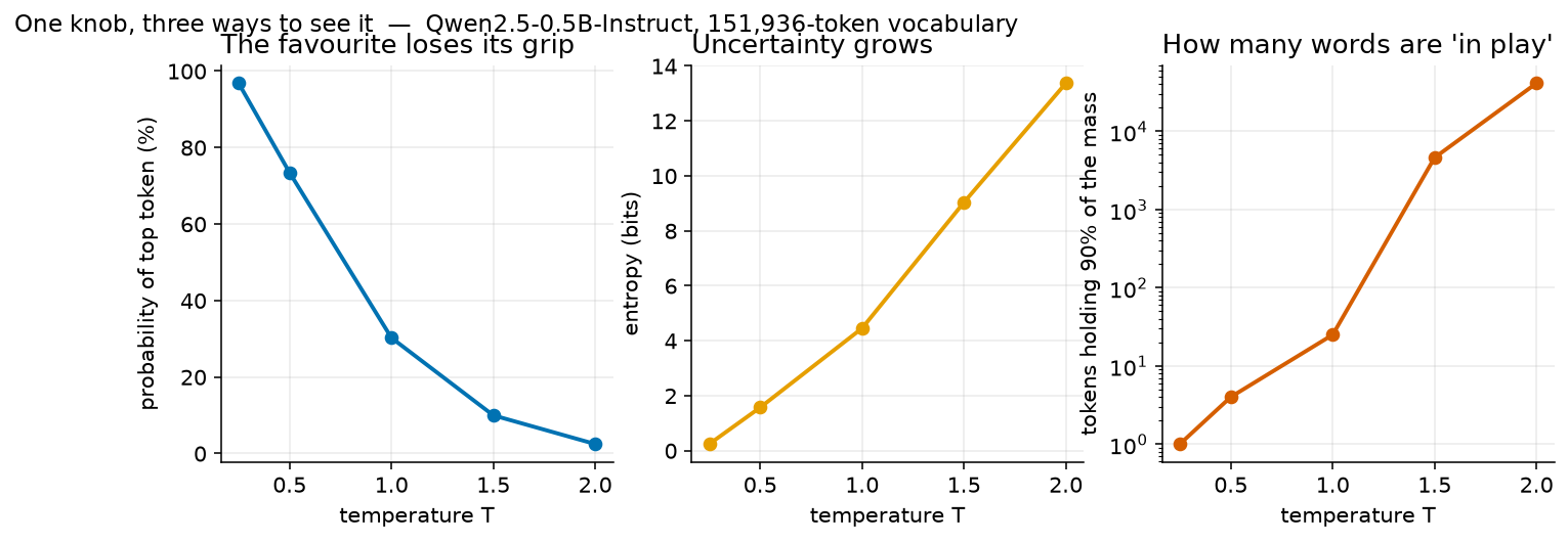
Figure 1:One dial, three ways to see it, all measured on Qwen2.5-0.5B-Instruct over its full
151,936-token vocabulary for the prompt The capital of France is. Left: the top token
' Paris' loses its grip, from 96.799% to 2.447%. Middle: uncertainty grows, from 0.237
bits to 13.367 bits, against a ceiling of 17.213 bits. Right: the number of tokens holding
90% of the probability climbs from 1 to 41,274; the vertical axis is logarithmic, so each
gridline is ten times the one below it, which is the only way to fit 1 and 41,274 on one chart.
Produced by lab/we2_softmax.py and lab/make_figures.py.
The right-hand chart has a logarithmic vertical axis, which is worth a sentence, because a logarithmic axis can mislead you if nobody says it is there. On an ordinary axis, equal steps up the page mean equal amounts added. On this one, equal steps up the page mean equal amounts multiplied, so the gridlines run 1, 10, 100, 1,000, 10,000. Without it the first four points would all be flat against the bottom of the chart and you would see nothing. Toolkit 13 covers reading axes from scratch.
5.5 Greedy or sampling, and where the creativity actually comes from
Intuition
Everything so far produced a distribution: a list of 151,936 probabilities that add to 1. But a model that is writing something has to put down one token and move on. Somewhere between the distribution and the text, a choice gets made, and that choice is a separate step with its own rules.
There are two rules in common use, and the difference between them is the thing people have been calling creativity.
The first rule is greedy decoding. Take the highest-probability token. Every time. No randomness anywhere. Run the same prompt a thousand times and you get the same output a thousand times. It is called greedy because it takes the biggest thing in front of it without thinking about what comes later, which is what “greedy” means when computer scientists use it about an algorithm. It is not a judgement about the quality of the output.
The second rule is sampling. Draw a token at random, but not evenly. Give each token a chance of being drawn equal to its probability. A token at 30.219% gets drawn about 30 times in 100. A token at 0.001% gets drawn about once in 100,000. Run the same prompt a thousand times and you get a thousand possibly different outputs.
Now the two ideas meet, and this is the payoff of the whole chapter. Temperature reshapes the distribution. Sampling is what turns a reshaped distribution into different text. Neither one does anything interesting without the other.
Set the temperature high and keep greedy decoding, and the output does not change at all, ever, because the ranking did not change and greedy only looks at the ranking. That single fact demolishes the creativity claim on its own. Turn the dial all the way to 2.0, and if the system is decoding greedily you get a character-for-character identical answer.
Set the temperature high and sample, and the output does change, because the unlikely
tokens now have a much larger share of the draw. At a sampler picks ' Paris' about
30 times in 100. At it picks ' Paris' about 2 times in 100, and the other 98 come
from a pool of tens of thousands of alternatives that includes a great deal of nonsense.
That is the honest sentence. It has two moving parts, and the marketing sentence has none.
The mathematics
Two rules, two formulas. Both are short.
Formula 5.7. Greedy decoding
1. In words. Pick the token whose probability is the largest. The answer is a position in the list, not a probability.
2. The formula.
3. The symbols.
| Symbol | How to say it out loud | What it means |
|---|---|---|
| “eye hat” | the answer: which token was chosen, given as its position in the list | |
| the hat | “hat” | a mark meaning “this is the one we picked” or “this is our estimate”, rather than a fixed known quantity |
| “equals” | the two sides are the same number | |
| “arg max” | short for “the argument that gives the maximum”. It returns the position of the biggest value, not the value. | |
| the underneath | “over i” | the position is being searched for among all the values of |
| “p sub i” | the probability of token |
4. Out loud. “ hat is the position at which is largest.”
The distinction between and is the only difficulty here, and it is worth one extra sentence. Given the list 0.665241, 0.244728, 0.090031, the max is 0.665241, because that is the biggest value. The arg max is 1, because the biggest value is in position 1. Greedy decoding wants the position, so it can look up which token lives there.
5. Worked, on the three made-up probabilities at .
Step 1, list the probabilities with their positions.
Position 1: 0.665241. Position 2: 0.244728. Position 3: 0.090031.
Step 2, find the largest value. Compare the first two: , so position 1 leads. Compare the leader with the third: , so position 1 still leads.
Step 3, report the position, not the value.
Step 4, repeat at , where the probabilities were 0.506480, 0.307196, 0.186324. The largest is 0.506480, in position 1. So again.
6. Check it. Greedy decoding gives the same answer at every temperature. That is not a coincidence and it is not a property of these particular numbers; it follows from Section 5.2, where you proved the ranking cannot change. If your arg max moved when you changed the temperature, you have made an arithmetic error somewhere upstream. This is the strongest available check on the work in this chapter, and it costs nothing to apply.
Formula 5.8. Sampling from a distribution
1. In words. Line the tokens up and give each one a stretch of a ruler as long as its probability, so the whole ruler is exactly 1 unit long. Throw a dart at the ruler, evenly, with no aim. Whichever token’s stretch the dart lands in is the token you drew.
2. The formula.
3. The symbols.
| Symbol | How to say it out loud | What it means |
|---|---|---|
| chosen | “chosen” | the answer: the position of the token you drew |
| “the smallest k such that” | the same construction as Formula 5.6: the first that satisfies the condition | |
| “kay” | a counter walking down the list | |
| “p one plus p two and so on up to p k” | the running total of probabilities from the top of the list down to position | |
| “is greater than or equal to” | the left side is at least as big as the right side | |
| “is less than or equal to” | the same sign the other way round: the left side is no bigger than the right side. The worked example below asks the question in this direction. See Toolkit 19. | |
| “you” | the dart: one random number between 0 and 1 | |
| “is distributed as” | the thing on the left is drawn according to the rule on the right | |
| Uniform | “uniform between nought and one” | every number between 0 and 1 is equally likely. This is what random.random() gives you. |
| the comma | “where” | it separates the rule from the description of |
4. Out loud. “The chosen token is the first one whose running total of probability reaches the random number , where is drawn evenly between 0 and 1.”
5. Worked, with five made-up dart throws. Use the three probabilities 0.665241, 0.244728 and 0.090031, which came from the made-up scores 2, 1 and 0. The five random numbers below are also made up for practice, so you can check the whole thing by hand.
Step 1, build the running totals once. These are the edges of the three stretches of ruler.
0.665241
So token 1 owns 0 up to 0.665241, token 2 owns 0.665241 up to 0.909969, and token 3 owns 0.909969 up to 1.
Step 2, take each dart throw in turn and find the first running total it does not exceed.
. Is ? Yes, so token 1.
. Is ? No. Is ? Yes, so token 2.
. Is ? No. Is ? No. Is ? Yes, so token 3.
. Below 0.665241, so token 1.
. Above 0.665241 and below 0.909969, so token 2.
Step 3, tally. Token 1 twice, token 2 twice, token 3 once.
6. Check it. The stretches must cover the ruler exactly once, with no overlaps and no gaps, so the last running total has to be 1. If it is not, your probabilities did not add to 1 and nothing after that is meaningful. The other check is on the long run: over many draws, the share going to each token should approach that token’s probability. Five draws is far too few to show that, and expecting five draws to land 2.0, 1.2 and 0.5 times is the classic mistake. Chapter 12 is about how far from the expected share a small sample can honestly wander.
Python
The next cell puts a number on the difference between greedy and sampling, using the measured
probability of ' Paris' at three temperatures.
# Cell 8. Greedy versus sampling, using the measured probability of ' Paris'.
# The probabilities are measured. The draw counts are simulated on this page.

random.seed(20260919)   # fixes the draws so your numbers match the book's exactly

measured_temperature = [0.25, 1.0, 2.0]                # three of the five measured settings
measured_paris_probability = [0.9679881930351257,      # P(' Paris') at T = 0.25
                              0.3021884262561798,      # P(' Paris') at T = 1.00
                              0.024472510442137718]    # P(' Paris') at T = 2.00

for position in range(3):
    random.seed(20260919)                              # reset, so each row starts from the same draws
    one_probability = measured_paris_probability[position]
    paris_count_sim = 0                                # a running count of simulated Paris draws
    for draw_number in range(1000):
        one_draw = random.random()                     # u, a number between 0 and 1
        if one_draw < one_probability:                 # Formula 5.8 with two outcomes
            paris_count_sim = paris_count_sim + 1
    print("T = %.2f   P(' Paris') = %7.3f%%   sampled ' Paris' %4d times in 1000"
          % (measured_temperature[position], one_probability * 100, paris_count_sim))
Output:
T = 0.25   P(' Paris') =  96.799%   sampled ' Paris'  967 times in 1000
T = 1.00   P(' Paris') =  30.219%   sampled ' Paris'  310 times in 1000
T = 2.00   P(' Paris') =   2.447%   sampled ' Paris'   26 times in 1000
Read those three rows next to what greedy decoding would have done. Greedy picks ' Paris'
1000 times out of 1000 in all three rows, because ' Paris' is the top-ranked token at all
three temperatures and greedy only looks at the ranking. The sampler picked it 967, 310 and 26
times.
That is the whole chapter in one table. The distribution changed enormously. The ranking did not change at all. Which of those two facts reaches the page depends entirely on the decoding rule, and the decoding rule is a separate setting from the temperature.
A note on the arithmetic of the simulation. With a probability of 0.302188 and 1000 draws you expect hits, and the simulation produced 310. Eight above expectation is unremarkable. Nothing is broken. Chapter 12 puts a proper interval around this kind of wobble and shows how wide it really is.
random.random() returns a number between 0 and 1 where every value is equally likely, which
is the from Formula 5.8. random.seed(20260919) fixes which numbers come out, and it is
reset at the start of each row so the three rows are compared on identical draws. Without a
seed, your counts would differ from the book’s and from each other, and neither of you would be
able to tell a real difference from noise.
Solution to Try it 5.5
What must be happening. Under greedy decoding the output cannot change when the temperature changes. Greedy takes the top-ranked token, temperature cannot alter the ranking, so the generated text is identical character for character at and at . The colleague is describing a change that the mechanism does not permit.
There are three plausible explanations and they are all testable.
The system is not really decoding greedily. Many tools label a setting “greedy” or “deterministic” and still sample when the temperature is above some threshold. The setting may not do what its label says.
Something else changed at the same time, such as the prompt, the system message, the model version or another sampling control like top-k or top-p.
Nothing changed and the impression is coming from reading different outputs on different days, which is a comparison with no control in it.
The measurement. Fix the prompt and the seed. Generate the output at and at with every other setting held identical. Compare the two strings character by character. If they are identical, greedy decoding is confirmed and the colleague’s impression has another source. If they differ, the system is sampling, whatever its documentation says, and now you know the real question to ask.
That is a controlled experiment: one variable moved, everything else held still. Chapter 9 builds this idea out properly.
Common mistakes
Dividing by the temperature after exponentiating instead of before. This is the most common error in the chapter. Temperature goes on the scores, inside the exponent. If you compute first and then divide that by , every result shrinks by the same factor, the renormalisation cancels it out, and you get the answer back no matter what you chose. How to spot it: your answers do not change when you move the dial.
Expecting the ranking to change. It cannot, at any positive temperature, ever. If your worked answer has a different token in front at than at , the arithmetic is wrong. How to spot it: check the first and last columns of your answer against the first and last of your scores.
Saying “temperature makes the model more creative”. Two separate settings are being blurred into one. Temperature reshapes the distribution; the decoding rule decides whether that reshaping ever reaches the page. Under greedy decoding, temperature changes nothing at all. How to spot it: ask what the decoding rule is. If the sentence does not mention it, the sentence is incomplete.
Forgetting the minus sign on the front of the entropy formula. Every logarithm of a probability is negative, so the sum is negative, and the minus sign is what makes the reported entropy positive. How to spot it: your entropy came out negative. Entropy is never negative.
Pressing
logand reporting a base-2 answer. Thelogkey is base 10 on nearly every calculator andlnis base . How to spot it: test the key on 8. must be 3. If you get 0.903, that is base 10, and you need to divide by .Comparing a top-eight probability with a full-vocabulary probability. At the eight-token version gives
' Paris'41.938% and the measured full-vocabulary answer is 30.219%. Both are correct answers to different questions. How to spot it: the two numbers agree closely at low temperature and diverge badly at high temperature, because the tail holds almost nothing when the distribution is sharp and a great deal when it is flat.Setting the temperature to zero. Formula 5.1 divides by , and division by zero has no answer, so is outside the formula. Systems that accept are quietly switching to greedy decoding instead. How to spot it: a tool that offers and a “greedy” option as though they were different things is describing one thing twice.
Treating the nine-tenths count as a smooth measure. It counts whole tokens, so it jumps. Between and it goes from 25 to 4,612 while entropy only doubles. How to spot it: you expected the two summaries to move together. They measure the same thing on different scales, and one of those scales is logarithmic.
Reading a logarithmic axis as though it were an ordinary one. On the right-hand panel of the three-views figure, a point twice as high up the page is ten times larger, not twice as large. How to spot it: check the axis labels. If they run 1, 10, 100, 1,000, the axis is logarithmic and the chart is compressing the top end.
What to remember
Temperature is one division, carried out on the model’s raw scores before those scores are exponentiated, and dividing by a number below 1 sharpens the distribution while dividing by a number above 1 flattens it. It cannot reorder the tokens, cannot add a candidate and cannot remove one, because doing the same thing to every score leaves the ranking exactly where it was. At it does nothing at all. The honest way to describe what it does is at the level of the whole distribution: on the measured run, entropy went from 0.237 bits to 13.367 bits, and the number of tokens holding 90% of the probability went from 1 to 41,274. Creativity is not in the dial; it is in the decoding rule that follows, and under greedy decoding the temperature changes nothing whatsoever.
Practice problems
Answers to the odd-numbered problems are in the answers appendix.
Every measured value you need is in this table, reproduced from
_research/00-lab-verified-findings.md section 2 and lab/out/we2_softmax.json. It is the
full-vocabulary measurement on Qwen2.5-0.5B-Instruct for the prompt
The capital of France is.
P(' Paris') | P(' ______') | P(':\n') | entropy | tokens holding 90% | |
|---|---|---|---|---|---|
| 0.25 | 96.799% | 2.670% | 0.220% | 0.237 bits | 1 |
| 0.50 | 73.430% | 12.195% | 3.500% | 1.568 bits | 4 |
| 1.00 | 30.219% | 12.315% | 6.597% | 4.450 bits | 25 |
| 1.50 | 9.949% | 5.469% | 3.607% | 9.031 bits | 4,612 |
| 2.00 | 2.447% | 1.562% | 1.143% | 13.367 bits | 41,274 |
Raw scores: ' Paris' 17.217289, ' ______' 16.319635, ':\n' 15.695457. Vocabulary size
151,936.
Warm-up: can you do the arithmetic
Divide the three scores 6, 3 and 0 by a temperature of 3. Write down the three answers.
Divide the same three scores by a temperature of 0.5. Say in one sentence why the answers got bigger when you divided.
Using a calculator’s
expkey, find , and to six decimal places.Two made-up scores, 1 and 0, at . Work out both probabilities, showing all four steps, and check they add to 1.
The same two scores at . Show all four steps.
The same two scores at . Show all four steps, then say which of the three settings gave the flattest answer.
Find , , and without a calculator, by asking “two to what power?” each time.
Find using Formula 5.4 and a base-10
logkey. Show both logarithms and the division.Work out the entropy of a distribution with two outcomes, each of probability 0.5. Show all four steps.
Work out the entropy of eight tokens that are all equally likely, so each has probability 0.125. Show all four steps.
Find for the sorted list 0.95, 0.03, 0.02, then for the sorted list 0.5, 0.45, 0.05. Show the running totals.
Convert the proportion 0.302188 into a percentage, and convert 96.799% back into a proportion.
Practice: can you apply it
Using the measured table, report how far P(
' Paris') falls between and , first in percentage points and then as “how many times smaller”. Say which of the two numbers you would put in a report, and why.The entropy ceiling for this vocabulary is bits. What share of that ceiling is the measured 13.367 bits at ? What share is the measured 0.237 bits at ?
The nine-tenths count is 4,612 at and 41,274 at . How many times larger is the second? Write one sentence a reader with no mathematics could understand.
Use Formula 5.2 and the measured score gap of 0.897654 to predict the ratio P(
' Paris') P(' ______') at . Then compute the same ratio directly from the measured percentages in the table, and explain the difference in the last digit.Take the three made-up probabilities, 0.665241, 0.244728 and 0.090031. Use Formula 5.3 with , which means squaring each one, then renormalising. Check your answer against Formula 5.1’s answer in the text.
Work out the three probabilities for the made-up scores 2, 1 and 0 at , then work out the entropy of your answer. Compare that entropy with the three-choice ceiling of 1.584963 bits, and say how close to flat this distribution is.
At the measured P(
' Paris') is 30.219%. If a system samples 100 tokens from this distribution, about how many would you expect to be' Paris'? Would exactly that many be surprising?The top eight measured tokens together hold 72.056% of the probability at . What share is left for the other 151,928 tokens? What does that tell you about using a top-eight chart to talk about the whole distribution?
A product lets a user set the temperature to 0. Explain in two sentences why Formula 5.1 has no answer at , and what the software is almost certainly doing instead.
Rewrite the sentence “temperature makes the model more creative” as a sentence that is true and that a non-technical colleague could act on. Your version must mention both the distribution and the decoding rule.
Stretch: can you reason with it
Prove, in your own words and in no more than five sentences, that no positive temperature can change which token the model ranks first. Use either Formula 5.2 or Formula 5.3, and say which one you used.
Between and , entropy roughly doubles, from 4.450 bits to 9.031 bits, while the nine-tenths count multiplies by about 184, from 25 to 4,612. Explain why two honest summaries of the same pair of distributions move at such different rates. Your answer should mention what a logarithm does to large numbers.
The chapter’s simulation, computing over the top eight tokens only, gives
' Paris'41.938% at , while the measured full-vocabulary answer is 30.219%. Reproduce the 41.938% from the measured numbers, using the fact that those eight tokens hold 72.056% of the probability. Then say which of the two numbers answers the question “how sure is the model that the next word is Paris”, and why.Suppose you raise the temperature without limit, so it becomes enormous. What do the 151,936 probabilities approach? What does the entropy approach? And what does the nine-tenths count approach? Give a number for each of the last two.
Now suppose you lower the temperature toward zero without ever reaching it. Answer the same three questions, and then explain the connection between your answer and greedy decoding.
Design an experiment that would falsify the claim “temperature makes the model more creative”. State the prompt, the settings you would hold fixed, the settings you would vary, what you would measure, and what result would count as the claim surviving. This is a question about the difference between a claim and a testable claim.
At , the 41,274 tokens holding 90% of the probability are 27.17% of the entire vocabulary. Is it fair to say the model is “considering” 41,274 words? Argue both sides in a short paragraph each, then state which version of the claim is measurable and which is not.
Two models are given the same prompt. Model A’s next-token distribution has entropy 0.237 bits and Model B’s has entropy 4.450 bits. The two models here are made up for practice; the two entropy figures are this chapter’s own measured values at and , borrowed so that you are reasoning about numbers you already trust. Which is riskier to sample from, and why is “riskier” a better word here than “less creative”? Name one measurement from a later chapter of this book that would tell you which model is actually better.