Chapter 12. Is that score real?
What you need before this chapter
An honest list. Nothing here is assumed; everything is either taught below or linked to a page that teaches it from zero.
You need to be able to divide one number by another, and to turn the answer into a percentage. You need to press the square root key on a calculator. That is the whole list of skills.
The Math Toolkit teaches each of these from nothing, with worked arithmetic. Open it in a second tab and go back to it whenever a symbol stops you.
| What this chapter uses | Where it is taught from zero |
|---|---|
| A letter standing for a number | Toolkit 1 |
| Subscripts, such as | Toolkit 2 |
| The fraction bar as division | Toolkit 4 |
| Square roots, and why a spread has one | Toolkit 9 |
| Sigma notation, “add these up” | Toolkit 10 |
| Percentages, decimals and percentage points | Toolkit 11 |
| Proportions and what “out of” means | Toolkit 12 |
| Reading a histogram | Toolkit 13 |
| Rounding, and rounding only once | Toolkit 16 |
| Inequality signs and interval notation, like | Toolkit 19 |
| The Greek letters this book uses | Toolkit 20 |
From earlier chapters you need one idea only: in Chapter 11 you gave a model a multiple-choice test and counted how many it got right. That count is where this chapter starts.
Setting up
Every piece of Python in this chapter runs on top of this one block. Run it first. Nothing else in the chapter imports anything.
# Every import this chapter needs, one per line, each with a note on what it is for.
import math                              # square roots, and rounding a number up
import numpy                             # fast arithmetic over long lists of numbers
import matplotlib.pyplot as pyplot       # draws every chart in this book

# The eight Okabe-Ito colours. They are chosen to stay apart from each other for readers
# with the common forms of colour vision deficiency. This book uses no other colours.
okabe_ito_blue = "#0072B2"               # the main series in most charts
okabe_ito_orange = "#E69F00"             # shaded intervals
okabe_ito_green = "#009E73"              # the improved method in a before-and-after pair
okabe_ito_vermillion = "#D55E00"         # the one value we actually measured
okabe_ito_sky_blue = "#56B4E9"           # histogram bars
okabe_ito_grey = "#999999"               # reference lines

# Chart settings used for every figure in this book.
pyplot.rcParams.update({
    "figure.dpi": 140,                   # dots per inch on screen, so the picture is sharp
    "savefig.dpi": 140,                  # dots per inch when the picture is written to a file
    "font.size": 11,                     # readable at the size these charts are printed
    "axes.spines.top": False,            # remove the top border of the plotting box
    "axes.spines.right": False,          # remove the right-hand border too
    "axes.grid": True,                   # faint gridlines help you read a value off the chart
    "grid.alpha": 0.25,                  # how dark those gridlines are, from 0 to 1
    "figure.facecolor": "white",         # white background on screen
    "savefig.facecolor": "white",        # white background in the saved file
    "savefig.bbox": "tight",             # trim the empty margin when the file is written
})
That is the whole setup. Three libraries and a colour scheme.
A number with nothing behind it
Drive almost anywhere in Kern County and somebody is selling you a percentage. A clinic on Truxtun Avenue advertises a success rate. A ballot measure poll on the local evening news reports the share of voters in favour, with the margin of error in type too small to read on a phone. A tutoring company promises a pass rate. The number is always printed large and always printed alone.
A percentage printed alone is a claim with nothing behind it. Not because it is a lie. Because one number cannot tell you the one thing you need, which is how much that number would have moved if the measurement had been taken slightly differently.
Here is a number of our own, and this one you can check.
In September 2026, on a laptop in Bakersfield, the course’s 0.5 billion parameter model,
Qwen2.5-0.5B-Instruct, sat a twenty-question multiple-choice test on introductory statistics.
The questions were written for this course. It was scored by the first procedure anyone reaches
for: compare the log-probability the model gives to each of the four letters A, B, C and D, and
take the largest. Name that procedure now, because Chapter 13 will show that a
different, equally defensible procedure moves the score. The scoring was deterministic, meaning
the model was not rolling any dice; run it again on the same twenty questions and it answers the
same way every time. Under the letter procedure it got 5 questions right out of 20, which is
25.0 percent.
So: the model scores 25 percent under that procedure. Print it on a slide and move on.
Except that you cannot, and the reason is not complicated. Those twenty questions are not the only twenty questions anybody could have asked about introductory statistics. They are twenty that a person sat down and wrote one afternoon. A different afternoon would have produced a different twenty. And a different twenty would have produced a different score.
You can see this without any statistics at all. Take the same twenty questions and split them down the middle. On the first ten the model got 2 right, which is 20 percent. On the last ten it got 3 right, which is 30 percent. Same model. Same day. Same settings. Two numbers, ten percentage points apart.
Which of those is the model’s accuracy?
Neither. That is the answer, and it is the whole chapter. The score is not a property of the model. It is a property of the model and the particular questions you happened to ask. Ask different questions and the number moves, even when nothing about the model has changed.
This chapter gives you three tools for saying how far it would move: a formula that is fast and sometimes wrong, a repair for when the fast formula breaks, and a simulation that needs no formula at all. By the end you will be able to replace “the model scored 25 percent” with a sentence that is actually true.
Learning objectives
By the end of this chapter you will be able to:
Explain why a benchmark score is a sample proportion, and why that makes it a quantity that moves, rather than a fixed property of a model.
Compute the standard error of an accuracy by hand, showing every step, and say in plain English what the resulting number means.
Build a 95 percent confidence interval two ways, using the Wald formula and using the bootstrap, and state the result as a sentence a non-specialist can act on.
Diagnose the case where the textbook interval returns an impossible accuracy above 100 percent, name the assumption that failed, and repair it with the Wilson interval.
Judge a reported benchmark number, including one you did not produce, by asking how many questions it rests on and how wide the honest interval around it would be.
This lesson at a glance
A score is one draw. 5 out of 20 is 25.0 percent, and the same model on a different twenty questions would have given a different number.
The wobble has a size you can compute. The standard error here is 0.0968, which is 9.68 percentage points, and it turns into an interval from 6.0 percent to 44.0 percent.
The textbook formula has assumptions. At 8 right out of 10 it returns an upper end of 1.0479, an accuracy of 104.79 percent, which cannot happen. The Wilson interval fixes it.
Twenty questions is not enough, and this is measurable. A benchmark that pins an accuracy to within 5 percentage points needs 385 questions, and the published recommendation is at least 1,000.
The vocabulary of this chapter
Every new word in this chapter is defined here, before it is used. Read the table once now. It will not all stick, and it is not meant to; it is here so that no word arrives unexplained.
| Word | What it means in one line |
|---|---|
| Population | Every question that could have been asked about the topic, not only the ones that were. |
| Sample | The questions that actually got asked. Here, twenty of them. |
| Sample proportion, | The share of the sample the model got right. Accuracy is a sample proportion. |
| Point estimate | A single number offered as an answer, with no range attached. “25 percent” is a point estimate. |
| Sampling variability | The amount a measurement moves around when you repeat it on a different sample. |
| Random variable | A quantity whose value depends on how a draw turns out. A benchmark score is one. |
| Standard error, | One number saying how far a measurement typically lands from the truth it is estimating. |
| Standard deviation | One number saying how spread out a list of values is: the typical distance of a value from the average of the list. |
| Confidence interval | Two numbers, a low end and a high end, offered in place of one number. |
| Margin of error | Half the width of a confidence interval. The “plus or minus” part. |
| Critical value, | A fixed multiplier that sets how confident the interval is. For 95 percent it is 1.96. |
| Wald interval | The textbook confidence interval for a proportion. Fast, and wrong at small sample sizes. |
| Wilson interval | A confidence interval for a proportion that can never fall outside 0 and 1. |
| Plus four interval | A one-line shortcut that lands close to Wilson. Add two correct and two wrong, then use the Wald formula. |
| Bootstrap | Building thousands of imitation tests out of the one test you have, to watch the score move. |
| Resample | One of those imitation tests. |
| With replacement | Drawing in a way that lets the same question come up twice, and lets others not come up at all. |
| Percentile | The value a given share of a sorted list sits below. The 2.5th percentile has 2.5 percent of the list below it. |
| Seed | A starting number for a random procedure, which makes the randomness repeat exactly. |
| Granularity | How coarse a measurement is. A twenty-question test can only move in steps of 5 percentage points. |
| Significant figures | How many digits in a number are actually carrying information. |
12.1 A score is one draw, not a fact
Intuition
Every September the Kern County Fair opens in Bakersfield, and somewhere on that fairground somebody is running a taste test. Two salsas, unlabelled, in small paper cups. Twenty people try both and say which one they prefer.
Suppose 13 of the 20 pick salsa A. That is 65 percent, and the stallholder writes it on a card: 65 percent prefer ours.
Now ask yourself a question that has nothing to do with salsa. If twenty different people had walked past that stall, would the number still have been 65 percent?
Almost certainly not. It might have been 60 percent. It might have been 75 percent. Nothing about the salsa would have changed. The only thing that changed is which twenty people happened to be standing there. The number on the card is not a fact about the salsa. It is a fact about the salsa and those twenty people, tangled together, and the card only reports one of them.
That is exactly the situation a benchmark score is in, and it catches people out because a computer feels so much more precise than a fairground. The model is deterministic. The scoring is deterministic. Run the same twenty questions through the same model a thousand times and you get 25.0 percent a thousand times. It is tempting to conclude that 25.0 percent is therefore a solid fact.
It is not, and the reason is that the randomness never lived in the model. It lived in the questions. Somebody had to choose twenty questions out of the enormous number of questions that could be asked about introductory statistics. That choice was a draw, and a different draw would give a different score, exactly as a different twenty fairgoers would give a different salsa number.
The rest of this chapter is about measuring the size of that effect. Before the measurement, four words.
The mathematics
Accuracy is a proportion. A proportion is a share of a whole, written as a number between 0 and
Before anything else, here is the formula that produces it, laid out in the six parts every formula in this book gets.
Formula 12.1: the sample proportion, which is what accuracy is
1. In words, with no symbols. Accuracy is the number of questions the model got right, divided by the number of questions you asked.
2. The formula.
3. Every symbol in it.
| Symbol | How to say it out loud | What it means |
|---|---|---|
| “p hat” | the answer: the accuracy you measured, as a number between 0 and 1 | |
| the hat, | “hat” | a mark meaning “measured from data”, as opposed to the true value you cannot see |
| “equals” | the thing on the left and the thing on the right are the same number | |
| “ex” | how many questions the model got right. A whole number. | |
| the fraction bar | “divided by” | divide the number on top by the number underneath |
| “divided by” | the same instruction as the fraction bar, written along one line instead of stacked. . This chapter uses it in every worked example. See Toolkit 4. | |
| “en” | how many questions were asked altogether |
4. How to say the whole thing out loud. “P hat equals x divided by n.” In longer English: “the measured accuracy is the number right divided by the number asked.”
5. Worked, on the real run. These are measurements, from lab/out/we6_eval.json.
Step 1, write down the two counts.
and
Step 2, divide the top by the bottom.
Step 3, turn the decimal into a percentage by multiplying by 100. This step is in Toolkit 11 if you want it from zero.
percent
So , which is 25.0 percent.
6. What going wrong looks like. A proportion must land between 0 and 1. If yours came out above 1, you divided the wrong way round; check that the smaller number is on top. There is also a sanity check specific to this test. Each question had four options, so a model that knew nothing and guessed at random would average one right in four, which is 25 percent. This model scored 25.0 percent. A score landing exactly on chance is a reason to distrust the measurement, and that suspicion is what Chapter 13 is built on. This chapter has a different job: even if the score were honest, how firm is it?
The hat is doing real work, so it is worth one more paragraph. There are two different things in play, and English gives them the same name.
The first is the model’s true accuracy: the share of the whole population of possible questions it would get right. Statisticians call this , with no hat. You will never see this number. You cannot ask infinitely many questions.
The second is the accuracy you measured, which is , with a hat. You can see this one. It is 0.25. It is an estimate of , and it is the only estimate you have.
The gap between and is what the whole chapter is about. Nobody can tell you what that gap is, because that would require knowing . But you can say how big it is likely to be, and that is a computation.
Python
Two short cells. The first one puts the real result into Python; the second splits it in half and shows the score moving.
Here is the graded run, one entry per question, in the order the questions were asked. A 1
means the model got that question right and a 0 means it did not. These twenty values are
copied out of lab/out/we6_eval.json.
# The real per-question result, from lab/out/we6_eval.json. 1 = right, 0 = wrong.
question_results = numpy.array([0, 0, 0, 0, 0, 0, 0, 1, 0, 1, 0, 1, 0, 0, 1, 0, 1, 0, 0, 0], dtype=float)

number_of_questions = len(question_results)          # len() counts the entries: 20
number_correct = int(question_results.sum())         # .sum() adds them up, so it counts the 1s
observed_accuracy = number_correct / number_of_questions   # the division from Formula 12.1

print("questions asked:", number_of_questions)
print("answered right :", number_correct)
print("accuracy       :", round(observed_accuracy * 100, 1), "percent")
Output:
questions asked: 20
answered right : 5
accuracy       : 25.0 percent
Four things in that cell are worth naming.
numpy.array(...) turns a plain list of numbers into a numpy array, which is a list that knows
how to do arithmetic on all of its entries at once. dtype=float stores the entries as decimals
rather than whole numbers, which matters because the average of five 1s and fifteen 0s needs to
come out as 0.25 and not be rounded to 0.
.sum() adds every entry. Because every entry is a 1 or a 0, adding them up counts the 1s.
int(...) wraps the result so it prints as 5 rather than 5.0.
round(observed_accuracy * 100, 1) multiplies by 100 to get a percentage, then rounds to 1
decimal place. Rounding happens here, at the print, and nowhere earlier. That is the house rule
from Toolkit 16: round once, at the end.
Now split the same twenty questions into two halves of ten and score each half on its own. Nothing about the model changes between the two halves. Only the questions change.
first_ten_results = question_results[0:10]      # entries 0 up to but not including 10
last_ten_results = question_results[10:20]      # entries 10 up to but not including 20

first_ten_accuracy = first_ten_results.sum() / 10
last_ten_accuracy = last_ten_results.sum() / 10

print("first ten questions:", int(first_ten_results.sum()), "right, which is",
      round(first_ten_accuracy * 100, 1), "percent")
print("last ten questions :", int(last_ten_results.sum()), "right, which is",
      round(last_ten_accuracy * 100, 1), "percent")
print("gap between halves :", round((last_ten_accuracy - first_ten_accuracy) * 100, 1),
      "percentage points")
Output:
first ten questions: 2 right, which is 20.0 percent
last ten questions : 3 right, which is 30.0 percent
gap between halves : 10.0 percentage points
question_results[0:10] is called slicing. It takes a piece of the array. The first number
is where to start counting, and Python starts counting at 0, not 1. The second number is where
to stop, and the entry at that position is not included. So [0:10] gives you the first ten
entries and [10:20] gives you the last ten.
The word points in that last line is deliberate and it is not a decoration. The two halves are 20 percent and 30 percent, and the gap between them is 10 percentage points, not 10 percent. Going from 20 percent to 30 percent is a rise of 10 percentage points and also a rise of 50 percent of the original value. Those are two different sentences about the same change. Toolkit 11 has the full version of this distinction. Reporters get it wrong constantly, and so will you unless you are deliberate.
Ten percentage points is an enormous gap. If two different labs published these two halves as two different benchmarks, one would report a model at 20 percent and the other a model at 30 percent, and they would be looking at exactly the same model on exactly the same day.
12.2 How far would the score move? The standard error
Intuition
You now believe that the score moves. The next question is the useful one: by how much?
Think about what makes a measurement of this kind unreliable, in ordinary terms, before any formula. Two things should come to mind, and both of them are right.
The first is how many questions you asked. Twenty people tasting salsa tells you less than two thousand people tasting salsa. This is the part everybody already knows. More questions, steadier number.
The second is less obvious and more interesting: how close the result is to a coin flip. Suppose a model gets every single question right, 20 out of 20. Ask another twenty questions of the same sort and you would expect it to do well again. There is not much room for the number to move; it is pinned against the ceiling. The same is true at the floor: a model that gets 0 out of 20 has nowhere to fall to.
But a model sitting at 10 out of 20, right in the middle, is the least predictable of all. Every question is genuinely up for grabs. A run of luck in either direction moves the total, and there is room on both sides for it to move into.
So the wobble is biggest in the middle and smallest at the ends, and it shrinks as you ask more questions. A single number that captures both of those effects is called the standard error, and the formula for it says exactly those two things in symbols.
One warning about the name, because it trips people up. “Standard error” sounds like somebody made a mistake. Nobody made a mistake. The word “error” here means the ordinary distance between a measurement and the truth it is estimating, which exists even when every step was done perfectly. A better name would be “typical distance from the truth”, and if it helps, read it that way every time.
The mathematics
Formula 12.2: the standard error of an accuracy
1. In words, with no symbols. The standard error of a score says how far that score would typically move if you had asked a different set of questions of the same size. It is built from two things: the share right multiplied by the share wrong, and the number of questions.
2. The formula.
3. Every symbol in it.
| Symbol | How to say it out loud | What it means |
|---|---|---|
| “the standard error” | the answer, in the same units as the accuracy | |
| “equals” | the two sides are the same number | |
| “the square root of” | what number, multiplied by itself, gives the number underneath. Everything under the long bar goes inside. See Toolkit 9. | |
| “p hat” | the accuracy you measured, from Formula 12.1 | |
| “minus” | subtract the thing on the right from the thing on the left | |
| “one minus p hat” | the share the model got wrong | |
| “brackets” | do what is inside the brackets before anything outside them | |
| the gap between and | “times” | multiply. Two things written side by side in maths means multiply them. See Toolkit 3. |
| the fraction bar | “divided by” | divide everything on top by everything underneath |
| “en” | how many questions were asked |
4. How to say the whole thing out loud. “The standard error is the square root of p hat times one minus p hat, all divided by n.”
The phrase “all divided by n” is doing important work. The division applies to the whole of , not to part of it. The fraction bar carries invisible brackets; so does the square root sign.
5. Worked, on the real run. and , from lab/out/we6_eval.json.
Every step is on a phone calculator.
Step 1, work out the share wrong.
Step 2, multiply the share right by the share wrong.
Step 3, divide that by the number of questions.
Step 4, take the square root. Press the key.
Round to four decimal places: .
Step 5, put it into units a person can use. Multiply by 100.
percentage points
6. What going wrong looks like. Four checks, and the fourth one surprises people.
The standard error must be positive. It is a square root of a positive number, so a negative answer means an arithmetic slip earlier.
It must get smaller as gets bigger. Try in step 3 and you get 0.00234375, whose square root is 0.0484, exactly half of 0.0968. Four times the questions, half the wobble.
It must be largest when . Try it: , which is bigger than , so the standard error at 50 percent is bigger than at 25 percent. That is the “coin flip is least predictable” idea, now visible in the arithmetic.
The square root made the number bigger, and that is correct. , and 0.0968 is much larger than 0.009375. The square root of any number between 0 and 1 is bigger than the number itself. If that looks like an error, it is not. Check it on 0.25: .
That value, 0.0968, is the most important number in the chapter, so here is what it means in a sentence you could say to somebody at a bus stop.
If you wrote a fresh twenty-question test of the same kind and ran the same model on it, the score you got would typically land about 9.68 percentage points away from the model’s true ability. Not always 9.68. Sometimes 2, sometimes 20. Typically about 9.68.
Against a measured score of 25.0 percent, a typical miss of 9.68 percentage points is enormous. It is more than a third of the score itself.
Python
The cell below does those five steps one line at a time. It would be shorter written as a single expression. It is not written that way on purpose, because a line you can read is worth more than a line you can admire.
share_wrong = 1 - observed_accuracy                          # step 1: the share got wrong
product_of_the_two_shares = observed_accuracy * share_wrong  # step 2: right times wrong
product_divided_by_n = product_of_the_two_shares / number_of_questions   # step 3: divide by n
standard_error = math.sqrt(product_divided_by_n)             # step 4: the square root

print("share right       :", observed_accuracy)
print("share wrong       :", share_wrong)
print("the two multiplied:", product_of_the_two_shares)
print("divided by n      :", product_divided_by_n)
print("standard error    :", round(standard_error, 4))
print("in points         :", round(standard_error * 100, 2), "percentage points")
Output:
share right       : 0.25
share wrong       : 0.75
the two multiplied: 0.1875
divided by n      : 0.009375
standard error    : 0.0968
in points         : 9.68 percentage points
Every printed line matches a step of the hand arithmetic above, in the same order, with the same digits. That is not a coincidence and it is worth pausing on. You did this on a calculator; the computer did the same thing; the numbers agree to the last place shown. The formula is not magic and the computer is not an oracle. They are doing the same four operations.
math.sqrt(...) is the square root. math is the library of ordinary mathematical operations
that came with Python, and sqrt is its name for the square root key on your calculator.
One note on the variable names. product_of_the_two_shares is a long name. It is long because
it says what the number is. A name like pq would be shorter and would tell you nothing three
weeks later. This course grades the long name.
12.3 From a wobble to a range: the Wald interval
Intuition
A standard error of 0.0968 is a real answer, but it is not yet a usable one. Nobody reads “the model scored 25 percent with a standard error of 0.0968” and knows what to do next.
What people can use is a range. Two numbers, a low one and a high one, with the honest claim that the truth is probably somewhere in between. That is a confidence interval, and building one from a standard error takes one multiplication and two additions.
Here is the idea behind the multiplication, without any theory. Sampling variability does not push a measurement out to its extreme every time. Most of the time the measurement lands close to the truth, sometimes it lands moderately far away, and only rarely does it land very far away. That pattern, common near the middle and rare at the edges, is the bell-shaped curve you have seen on charts your whole life.
The useful fact about that curve is that it comes with a fixed conversion table. Reach out 1.96 standard errors on each side of your measurement and you have covered the middle 95 percent of the curve. Reach out 2.58 standard errors and you have covered 99 percent. Reach out 1.00 and you have covered about 68 percent.
This book uses 1.96 and nothing else. The number is called a critical value and it is written , said “z star”. You do not have to derive it. You do have to know that 1.96 means “95 percent” and that it is not something you choose to make your results look better.
So the recipe is: take your measurement, work out the standard error, multiply it by 1.96, and go that far in each direction. The width you get is the price of honesty. If it is uncomfortably wide, the interval is not being pessimistic. Your test was small.
The mathematics
Formula 12.3: the Wald confidence interval for an accuracy
1. In words, with no symbols. Take the accuracy you measured. Go out the same distance above it and below it, where that distance is 1.96 times the standard error. Those two numbers are the ends of the interval.
2. The formula.
3. Every symbol in it.
| Symbol | How to say it out loud | What it means |
|---|---|---|
| “p hat” | the accuracy you measured, from Formula 12.1 | |
| ± | “plus or minus” | do the calculation twice, once subtracting and once adding. You get two answers, and they are the two ends of the interval. |
| “z star” | the critical value. 1.96 for 95 percent confidence, always, in this book. | |
| the star, | “star” | part of the name of the symbol. It does not mean multiply and it is not an exponent. |
| “times” | multiply | |
| “the standard error” | from Formula 12.2 |
4. How to say the whole thing out loud. “P hat, plus or minus z star times the standard error.” In longer English: “the accuracy you measured, give or take one point nine six standard errors.”
5. Worked, on the real run. , , from Worked example 12.1.
Step 1, multiply the standard error by the critical value.
Round to four places: 0.1897. This is the margin of error.
Step 2, subtract it from the accuracy to get the low end.
Step 3, add it to the accuracy to get the high end.
Step 4, convert both ends to percentages.
, which rounds to 6.0 percent
, which rounds to 44.0 percent
Step 5, write it in interval notation, which is two numbers in round brackets with a comma between them. See Toolkit 19.
6. What going wrong looks like. Three checks.
The measurement must sit exactly in the middle. Here and . Equal on both sides, as it must be. If your two gaps differ, you subtracted or added the wrong thing.
The low end must be below the high end. If it is not, you swapped the plus and the minus.
A very wide interval is not an arithmetic mistake. It is the answer. Thirty-eight percentage points of width is what twenty questions buys you.
Now say the result out loud, because the sentence is the point of the whole section.
The model did not score 25 percent. The model scored somewhere around 6 percent to 44 percent, and the single best guess inside that range is 25 percent.
Read those two ends again. Six percent is a model that has learned almost nothing. Forty-four percent is a model that is meaningfully better than guessing. Twenty questions cannot tell those two stories apart. That is not a failure of the arithmetic; the arithmetic worked. It is a failure of the test.
Python
z_star = 1.96                                          # the 95 percent critical value
margin_of_error = z_star * standard_error              # step 1: how far to reach each way
wald_lower_end = observed_accuracy - margin_of_error   # step 2: go down
wald_upper_end = observed_accuracy + margin_of_error   # step 3: go up
interval_width = wald_upper_end - wald_lower_end       # how wide the answer turned out to be

print("z star         :", z_star)
print("margin of error:", round(margin_of_error, 4))
print("lower end      :", round(wald_lower_end * 100, 1), "percent")
print("upper end      :", round(wald_upper_end * 100, 1), "percent")
print("width          :", round(interval_width * 100, 1), "percentage points")
Output:
z star         : 1.96
margin of error: 0.1898
lower end      : 6.0 percent
upper end      : 44.0 percent
width          : 38.0 percentage points
The margin prints as 0.1898 rather than the 0.1897 you got by hand, for the reason in the
warning above: Python carried all the digits of the standard error and you carried four. Both
routes land on 6.0 percent and 44.0 percent, which are the numbers in lab/out/we6_eval.json.
The last line is the one to sit with. Thirty-eight percentage points. An interval that wide covers almost everything a model could plausibly be. It contains 25 percent, which is what blind guessing gets, and it also contains 40 percent, which would be a model that knows something. Twenty questions did not separate those two possibilities, and no amount of care in the arithmetic will make it do so.
Notice that the code has no formula in it. It has a multiplication, two subtractions and an addition, on lines you can read one at a time. The formula was the hard part and you already did it by hand.
One more thing about the width. It is exactly twice the margin of error, because the interval reaches the same distance in both directions: , which is 38.0 percentage points after rounding. That is a free check on the two ends, and if your width is not twice your margin, one of the two ends is wrong.
12.4 The interval that runs past 100 percent
Intuition
You have now met the thing this section is about, in Try it 12.2. A formula every textbook prints, applied carefully, returned an accuracy above 100 percent.
Most books handle this by quietly chopping the interval off at 1 and moving on. This book does not, because the situation is worth more than a fix. It is the clearest example in the whole course of something students are rarely told plainly:
A formula is a tool with a range of use, not a guarantee.
Formula 12.3 was built by assuming that the wobble in a score follows that smooth bell-shaped curve from section 12.3. The bell curve is a beautiful description of many things, and one of its features is that it never stops. It stretches out forever in both directions, assigning smaller and smaller probabilities to values further and further away.
An accuracy cannot do that. An accuracy lives on a short leash between 0 and 1, and when the measurement is already near one end and the sample is small, the bell curve does not fit. It drapes off the edge of the world. The formula, which does not know where the edge is, reports what it sees.
You can feel when this is coming. The bell approximation works when there are a decent number of right answers and a decent number of wrong answers. A common rule of thumb is at least ten of each, which at 8 right out of 10 fails badly: two wrong answers, not ten. Small samples near an edge break it. Our real run, 5 right and 15 wrong out of 20, also fails the rule of thumb, which is worth knowing before you trust the interval from section 12.3 too far.
The repair is a formula called the Wilson interval. It does the same job and it can never produce an impossible answer, because of how it is built rather than because anything gets trimmed. It is slightly more arithmetic. It is not harder arithmetic.
There is also a one-line shortcut called the plus four interval, which lands very close to Wilson and can be done in your head on a good day. You will do all three.
The mathematics
First, watch the failure happen in full. Every step, by hand.
That is the set piece. Do not let anybody tell you it is a technicality. A formula returning 104.79 percent for a quantity that cannot exceed 100 percent is the formula telling you, as loudly as it can, that it does not apply here.
Now the repair.
Formula 12.4: the Wilson confidence interval for an accuracy
1. In words, with no symbols. The same job as the Wald interval, done in a way that cannot produce an impossible answer. It pulls the centre of the interval away from the score you measured and towards the middle, by an amount that shrinks as you ask more questions, and both of its ends always land between 0 and 1.
2. The formula. It comes in two pieces which you work out separately and then combine.
3. Every symbol in it.
| Symbol | How to say it out loud | What it means |
|---|---|---|
| “centre” | the middle of the interval. It is not . It is shifted towards 0.5. | |
| “half width” | how far the interval reaches on each side of the centre | |
| “ex” | how many questions the model got right | |
| “en” | how many questions were asked | |
| “p hat” | the measured accuracy, | |
| “z star” | the critical value, 1.96 for 95 percent | |
| “z star squared” | ||
| the raised 2 | “squared” | multiply the thing by itself. See Toolkit 5. |
| “z star squared over two” | . Adding this to is what shifts the centre. | |
| “z star squared over four” | ||
| “the square root of” | everything under the long bar goes inside | |
| “plus” | add | |
| ± | “plus or minus” | do it twice, once subtracting and once adding |
| the fraction bars | “divided by” | divide the top by the bottom |
4. How to say the whole thing out loud. “The centre is the number right plus half of z star squared, all divided by the number of questions plus z star squared. The half-width is z star divided by that same bottom, multiplied by the square root of the accuracy times one minus the accuracy times the number of questions, plus a quarter of z star squared. The interval is the centre plus or minus the half-width.”
That is a mouthful. It is nine small steps and none of them is harder than dividing.
5. Worked, on the same 8 out of 10 (made up for practice).
Step 1, square the critical value.
Step 2, build the bottom, which both pieces share.
Step 3, build the top of the centre. Half of is , so
Step 4, divide to get the centre.
Step 5, build what goes under the square root. Three sub-steps:
, and
Step 6, take the square root.
Step 7, work out the multiplier in front of the root.
Step 8, multiply to get the half-width.
Step 9, subtract and add.
, which rounds to
, which rounds to
6. What going wrong looks like. Both ends must land between 0 and 1, for every possible and every possible . That is the entire reason this formula exists, so an end outside that range means an arithmetic slip, not a broken formula. Second check: the centre must sit between and 0.5. Here 0.7167 sits between 0.5 and 0.8, which is right.
Put the two side by side. This comparison is the one to carry out of the chapter.
| 8 right out of 10, 95 percent | low end | high end | inside 0 and 1? |
|---|---|---|---|
| Wald, Formula 12.3 | 0.5521 | 1.0479 | no |
| Wilson, Formula 12.4 | 0.4902 | 0.9433 | yes |
Look at what Wilson did, because it is not what people expect. It did not take the Wald interval and trim the top off at 1. It moved both ends down. The low end fell from 0.5521 to 0.4902.
That is the formula saying something sensible about the world. A model that got 8 of 10 right is more likely to be a middling model that had a good morning than an outstanding model that had a bad one, because there are more middling models than outstanding ones. With only ten questions, that tilt matters, and Wilson accounts for it. With a thousand questions the tilt would be tiny and Wald and Wilson would nearly agree.
Now the shortcut, for when you have no computer.
Formula 12.5: the plus four interval
1. In words, with no symbols. Pretend you asked four more questions than you did, and that the model got two of them right and two of them wrong. Then use the ordinary Wald formula on those pretend numbers. That small nudge towards the middle is enough to stop the interval escaping past 0 or 1 in almost every case.
2. The formula.
3. Every symbol in it.
| Symbol | How to say it out loud | What it means |
|---|---|---|
| “p tilde” | the pretend accuracy after adding two right and two wrong | |
| the tilde, | “tilde”, rhymes with “gilded” | a wavy mark, used here to mean “adjusted”. It is a different mark from the hat, and a different number. |
| “ex” | how many questions the model actually got right | |
| “en” | how many questions were actually asked | |
| “x plus two” | the pretend number right | |
| “n plus four” | the pretend number of questions | |
| “z star” | 1.96, as before | |
| ± | “plus or minus” | do it twice, subtracting then adding |
| “the square root of” | everything under the bar |
4. How to say the whole thing out loud. “P tilde is x plus two, divided by n plus four. Then the interval is p tilde, plus or minus z star times the square root of p tilde times one minus p tilde, all divided by n plus four.”
5. Worked, on the same 8 out of 10 (made up for practice).
Step 1, add two to the number right.
Step 2, add four to the number of questions.
Step 3, divide to get the pretend accuracy.
Step 4, the share wrong.
Step 5, multiply the two shares.
Step 6, divide by the pretend number of questions.
Step 7, take the square root.
Step 6 was rounded to six decimal places before you took this root. Carry it unrounded, as 0.0145773, and the root is 0.120736 instead. That is the value the computer prints below, so carry 0.120736 into the next step. The two routes agree to four decimal places at the end, which is all this answer is reported to.
Step 8, multiply by 1.96.
Step 9, subtract and add.
, which rounds to
, which rounds to
6. What going wrong looks like. Compare the answer with Wilson, which is what the shortcut is imitating. Wilson gave and plus four gives . The two ends differ by about 1 percentage point each, which is far less than the width of the interval. If your plus four answer is nowhere near your Wilson answer, one of the two has an arithmetic slip in it. And unlike Wald, the upper end is now safely under 1.
Three methods, one made-up result. Here they are together.
| 8 right out of 10, 95 percent | low end | high end | usable? |
|---|---|---|---|
| Wald, Formula 12.3 | 0.5521 | 1.0479 | no, the high end is impossible |
| Wilson, Formula 12.4 | 0.4902 | 0.9433 | yes, this is the one to report |
| Plus four, Formula 12.5 | 0.4776 | 0.9509 | yes, and you can do it on paper |
One more interval is owed to you before this section closes. Section 12.3 published a Wald interval for our own measurement, 5 right out of 20, and then the rule of thumb above said that 5 right and 15 wrong is not enough of each. A book that tells you to switch to Wilson when the rule of thumb fails has to do it on its own headline number.
Python
Three cells, each doing one method, with prose between them. No helper functions, because a function you have to scroll up to read is worse here than four lines you can see.
First the failure, so you can watch a computer produce an impossible number without complaining.
small_number_correct = 8                # made up for practice
small_number_of_questions = 10          # made up for practice
small_accuracy = small_number_correct / small_number_of_questions
small_share_wrong = 1 - small_accuracy
small_standard_error = math.sqrt(small_accuracy * small_share_wrong / small_number_of_questions)
small_margin_of_error = 1.96 * small_standard_error
small_wald_lower_end = small_accuracy - small_margin_of_error
small_wald_upper_end = small_accuracy + small_margin_of_error

print("accuracy       :", small_accuracy)
print("standard error :", round(small_standard_error, 6))
print("margin of error:", round(small_margin_of_error, 6))
print("lower end      :", round(small_wald_lower_end, 4))
print("upper end      :", round(small_wald_upper_end, 4))
print("is the upper end above 1?", small_wald_upper_end > 1)
Output:
accuracy       : 0.8
standard error : 0.126491
margin of error: 0.247923
lower end      : 0.5521
upper end      : 1.0479
is the upper end above 1? True
Every number matches Worked example 12.3. The last line is the important one. > is the
“greater than” sign from
Toolkit 19, and a comparison like this
gives back True or False rather than a number. Python answered True: the formula produced
an accuracy above 100 percent and reported it without hesitation, because nothing in the formula
knows that accuracies stop at 1. The software will not catch this for you. You will.
Now Wilson, in the nine steps you did by hand.
z_star_squared = 1.96 * 1.96                                      # step 1
wilson_bottom = small_number_of_questions + z_star_squared        # step 2
wilson_centre = (small_number_correct + z_star_squared / 2) / wilson_bottom      # steps 3 and 4
wilson_under_the_root = small_accuracy * small_share_wrong * small_number_of_questions + z_star_squared / 4   # step 5
wilson_half_width = (1.96 / wilson_bottom) * math.sqrt(wilson_under_the_root)    # steps 6, 7, 8
wilson_lower_end = wilson_centre - wilson_half_width              # step 9, down
wilson_upper_end = wilson_centre + wilson_half_width              # step 9, up

print("z star squared:", round(z_star_squared, 4))
print("bottom        :", round(wilson_bottom, 4))
print("centre        :", round(wilson_centre, 6))
print("under the root:", round(wilson_under_the_root, 4))
print("half width    :", round(wilson_half_width, 6))
print("lower end     :", round(wilson_lower_end, 4))
print("upper end     :", round(wilson_upper_end, 4))
print("is the upper end above 1?", wilson_upper_end > 1)
Output:
z star squared: 3.8416
bottom        : 13.8416
centre        : 0.716738
under the root: 2.5604
half width    : 0.226581
lower end     : 0.4902
upper end     : 0.9433
is the upper end above 1? False
False this time. Same data, same confidence level, an answer that exists.
Every printed value has a matching step in the hand calculation: 3.8416, 13.8416, 0.716738, 2.5604, 0.226581, 0.4902, 0.9433. Seven numbers, seven matches. If one of yours disagrees, that tells you which step to redo.
Finally the shortcut, which is four lines.
plus_four_correct = small_number_correct + 2          # pretend two more right answers
plus_four_total = small_number_of_questions + 4       # pretend four more questions
plus_four_accuracy = plus_four_correct / plus_four_total
plus_four_standard_error = math.sqrt(plus_four_accuracy * (1 - plus_four_accuracy) / plus_four_total)
plus_four_lower_end = plus_four_accuracy - 1.96 * plus_four_standard_error
plus_four_upper_end = plus_four_accuracy + 1.96 * plus_four_standard_error

print("pretend correct :", plus_four_correct)
print("pretend total   :", plus_four_total)
print("pretend accuracy:", round(plus_four_accuracy, 6))
print("standard error  :", round(plus_four_standard_error, 6))
print("lower end       :", round(plus_four_lower_end, 4))
print("upper end       :", round(plus_four_upper_end, 4))
Output:
pretend correct : 10
pretend total   : 14
pretend accuracy: 0.714286
standard error  : 0.120736
lower end       : 0.4776
upper end       : 0.9509
0.4776 and 0.9509, against Wilson’s 0.4902 and 0.9433. About a percentage point apart at each end, on an interval more than 45 percentage points wide. For a quick check in a meeting, that is close enough. For a published result, use Wilson.
12.5 The bootstrap: what if the questions had been different?
Intuition
Everything so far came out of a formula, and the last section showed you that a formula carries assumptions you may not have noticed. So here is a completely different route to the same question, one that assumes almost nothing.
Start from the thing you actually want. You want to know what would have happened if the test had contained a different twenty questions. The honest way to find out is to write another twenty questions, run the model, and see. Then do it again. Do it ten thousand times and you would know the answer exactly.
Nobody has ten thousand question banks. So here is the trick, and it is one of the best ideas in twentieth-century statistics.
Build the new tests out of the old one.
Put your twenty questions in a hat, with the model’s result for each one already written on it. Draw one out, write down what the model scored on it, and put it back in the hat. Draw again. Do that twenty times. You now have a twenty-question test. It is not the original test: some questions turned up twice, some three times, and some never turned up at all. Score it.
That is one imitation test, called a resample. Do it ten thousand times and you have ten thousand scores. Look at how they spread out, and that spread tells you how much your one real score could have wobbled.
The part people stumble on is putting the question back in the hat. It feels like cheating. Why would you let the same question appear twice?
Because if you did not put it back, you would draw all twenty questions exactly once, every single time, and every imitation test would be the original test with the questions in a different order. Every score would be 25 percent. You would learn nothing. Putting it back is what creates the variety, and the variety is the entire point. It stands in for the variety you would have got from a genuinely new set of questions.
There is one honest limit, and this book states it rather than hiding it. The bootstrap can only reshuffle the information you already collected. If your twenty questions happened to miss an entire topic, no amount of resampling will tell you about that topic. Resampling reveals how shaky a small sample is. It does not make a small sample into a large one.
The mathematics
There are two numbers to get out of ten thousand resampled scores: an interval, and a measure of spread. Here are both.
Formula 12.6: the bootstrap percentile interval
1. In words, with no symbols. Sort all of your imitation scores from smallest to largest. Cut off the lowest 2.5 percent and the highest 2.5 percent. What is left in the middle is your 95 percent interval, and its two ends are the two numbers you report.
2. The formula.
3. Every symbol in it.
| Symbol | How to say it out loud | What it means |
|---|---|---|
| “p hat star” | an accuracy computed on a resample rather than on the real test. The star marks it as an imitation. | |
| the star, | “star” | a mark meaning “this came from a resample”. It does not mean multiply. |
| “capital B” | how many resamples you take. In this book . | |
| “p hat star, bracket r” | the -th smallest of the resampled accuracies, after sorting them. The round brackets around the subscript mean the list has been sorted. | |
| “ceiling” | round up to the next whole number. , and . | |
| 0.025 | “nought point nought two five” | 2.5 percent, the share left below the low end |
| 0.975 | “nought point nine seven five” | 97.5 percent, the share left below the high end |
| the space between 0.025 and | “times” | multiply |
| the outer brackets and the comma | “the interval from, to” | they hold the two ends |
4. How to say the whole thing out loud. “The interval runs from the resampled accuracy two and a half percent of the way up the sorted list, to the resampled accuracy ninety-seven and a half percent of the way up.”
5. Worked, in two parts.
Part one: one resample, by hand (made up for practice). Take an invented five-question test where the model got questions 1, 2 and 4 right and questions 3 and 5 wrong. Write that as
The real score is .
Step 1, draw five question numbers at random from 1 to 5, putting each one back after drawing. Suppose you draw 2, 2, 5, 1, 4.
Step 2, look up what the model scored on each of those.
question 2 was right, so 1
question 2 again, so 1
question 5 was wrong, so 0
question 1 was right, so 1
question 4 was right, so 1
Step 3, add them and divide.
, and
One resample, one number, and it came out at 0.8 instead of the real 0.6. Question 3 never got drawn and question 2 got drawn twice. That is what “with replacement” produces.
Part two: reading the ends off ten thousand of them. This is the part you do by hand.
Step 1, write down how many resamples you took. .
Step 2, find the rank of the low end. . It is already a whole number, so the ceiling leaves it at 250.
Step 3, find the rank of the high end. .
Step 4, sort the ten thousand resampled accuracies from smallest to largest and read off the 250th value and the 9,750th value.
On the real run, seeded 20260912, those two values are 0.05 and 0.45.
6. What going wrong looks like. Both ranks must be whole numbers between 1 and , and the low rank must be smaller than the high one. The interval itself lands inside 0 and 1 automatically, because every resampled score is a real score on a real number of questions; this method cannot return 104.79 percent. Then compare with the formula. Wald gave and the bootstrap gives . Two completely different routes landing within about one percentage point of each other at both ends is a strong sign that neither has an error in it.
Formula 12.7: the bootstrap standard error
1. In words, with no symbols. Take all of your imitation scores, work out their average, then work out how far each one sits from that average. Square those distances so the negatives do not cancel the positives, average the squares, and take the square root at the end to get back into the original units. The answer is the standard error, measured rather than predicted.
2. The formula.
3. Every symbol in it.
| Symbol | How to say it out loud | What it means |
|---|---|---|
| “the bootstrap standard error” | the answer | |
| “the square root of” | everything under the long bar | |
| “one over B” | multiplying by one over B is the same as dividing by B, which is how you take an average | |
| “sum”, the Greek capital letter sigma | add up everything to the right of it, once for each value of the counter. See Toolkit 10. | |
| “bee” | the counter. It takes the value 1, then 2, then 3, and so on. | |
| underneath the sigma | “b equals one” | where the counter starts |
| above the sigma | “capital B” | where the counter stops. Here, 10,000. |
| “p hat star sub b” | the accuracy of resample number | |
| “p bar star” | the average of all resampled accuracies. A bar on top means “the average of”. | |
| the bar, | “bar” | a flat line on top, meaning “average”. It is a third mark, different from the hat and the tilde. |
| “all squared” | multiply the bracket by itself, after working out what is inside | |
| “minus” | subtract |
4. How to say the whole thing out loud. “The bootstrap standard error is the square root of one over B, times the sum, as b goes from one to B, of the square of resample b’s accuracy minus the average resampled accuracy.”
Shorter, and the version to remember: “the square root of the average squared distance from the average.”
5. Worked, on four made-up resamples. Ten thousand will not fit on a page, so here are four invented ones, chosen so the arithmetic is clean.
Suppose your four resampled accuracies are 0.20, 0.25, 0.30, 0.25.
Step 1, find the average.
, and
So .
Step 2, find each distance from the average.
Step 3, square each distance. Squaring turns the negative into a positive, which is the reason this step exists.
Step 4, add the squares.
Step 5, divide by how many there are.
Step 6, take the square root, which puts the answer back into the units of an accuracy.
6. What going wrong looks like. The distances in step 2 must add to zero, every time: . That is a free check on your average, and if it does not come out at zero you computed the average wrong. The final answer must be positive, and it must be smaller than the full spread of your values. Above all, compare it with Formula 12.2. On the real run, Formula 12.2 predicted 0.0968, and the ten thousand resamples measured 0.0974. Two different methods, agreeing to within 0.0006. The formula was not making anything up.
Python
The bootstrap is five lines of Python, and the loop in the middle is the whole idea.
random_generator = numpy.random.default_rng(20260912)   # the seed, so this repeats exactly
bootstrap_accuracies = []                               # an empty list to collect the scores in

for one_resample in range(10000):                       # do the next two lines 10,000 times
    resampled_results = random_generator.choice(question_results, size=20, replace=True)
    bootstrap_accuracies.append(resampled_results.mean())

bootstrap_accuracies = numpy.array(bootstrap_accuracies)   # turn the list into a numpy array

print("how many resamples:", len(bootstrap_accuracies))
print("first three scores:", bootstrap_accuracies[0:3])
print("mean of all 10,000:", round(float(bootstrap_accuracies.mean()) * 100, 1), "percent")
print("standard deviation:", round(float(bootstrap_accuracies.std()) * 100, 2), "percentage points")
Output:
how many resamples: 10000
first three scores: [0.25 0.15 0.35]
mean of all 10,000: 24.8 percent
standard deviation: 9.74 percentage points
Line by line.
numpy.random.default_rng(20260912) makes a random number generator and fixes its seed at
20260912. Because the seed is fixed, your first three scores will be 0.25, 0.15 and 0.35 as
well, on your machine, today or in five years. That is the point of seeding.
for one_resample in range(10000): starts a loop that runs the indented lines below it ten
thousand times. range(10000) produces the counting numbers 0 up to 9,999. The variable
one_resample holds the current count; nothing inside the loop uses it, and it still gets a
readable name.
random_generator.choice(question_results, size=20, replace=True) is the hat. It draws 20
entries from question_results. replace=True is the phrase “with replacement”. Change it to
replace=False and every draw would return all twenty questions exactly once, every resample
would score 25 percent, and the whole exercise would collapse.
.mean() averages the twenty drawn results. Because they are all 1s and 0s, the average is
the proportion right, which is the resample’s accuracy.
.append(...) adds that one number to the end of the list.
.std() is the standard deviation, which is Formula 12.7 done by the computer.
Now read the output, because three of those four lines say something.
The first three resamples came out at 25 percent, 15 percent and 35 percent. Nothing about the model changed between them. Nothing about the scoring changed. The only thing that changed was which questions got drawn out of the hat. That is sampling variability, visible in three numbers.
The mean of all ten thousand is 24.8 percent, close to the 25.0 percent we measured. The bootstrap distribution centres on your measurement, not on the truth. It cannot tell you where the truth is; it can only tell you how far things move.
The standard deviation is 9.74 percentage points. Formula 12.2 predicted 9.68 percentage points from a completely different starting point. The two disagree by 0.06 percentage points.
Next, the interval.
lower_edge = numpy.percentile(bootstrap_accuracies, 2.5)    # 2.5 percent of scores are below this
upper_edge = numpy.percentile(bootstrap_accuracies, 97.5)   # 97.5 percent of scores are below this

print("lower edge:", round(float(lower_edge) * 100, 1), "percent")
print("upper edge:", round(float(upper_edge) * 100, 1), "percent")
Output:
lower edge: 5.0 percent
upper edge: 45.0 percent
numpy.percentile(values, 2.5) sorts the values and finds the one with 2.5 percent of the list
below it. That is Formula 12.6, steps 1 to 4, in one line.
Put the two methods side by side one last time.
| method | low end | high end | width |
|---|---|---|---|
| Wald formula, Formula 12.3 | 6.0% | 44.0% | 38.0 points |
| Bootstrap percentile, Formula 12.6 | 5.0% | 45.0% | 40.0 points |
Both are in lab/out/we6_eval.json. They were computed by completely different means: one from
a square root and a multiplication, the other from ten thousand simulated tests. They agree to
within one percentage point at each end.
The simulation
Do the resampling yourself. Press Resample once about ten times and watch the last score jump around. Then press Resample 1000 and the whole pile appears at once.
The strip along the top shows which of the twenty questions the current resample happened to draw. Some appear twice. Some do not appear at all. That is the hat.
Two readouts are worth watching in particular. Scores seen counts how many different values have turned up; it will stop climbing long before you expect it to, for a reason that is section 12.6. Not 25% counts the share of resamples that came out at anything other than the score we actually measured, and it will settle near 80 percent.
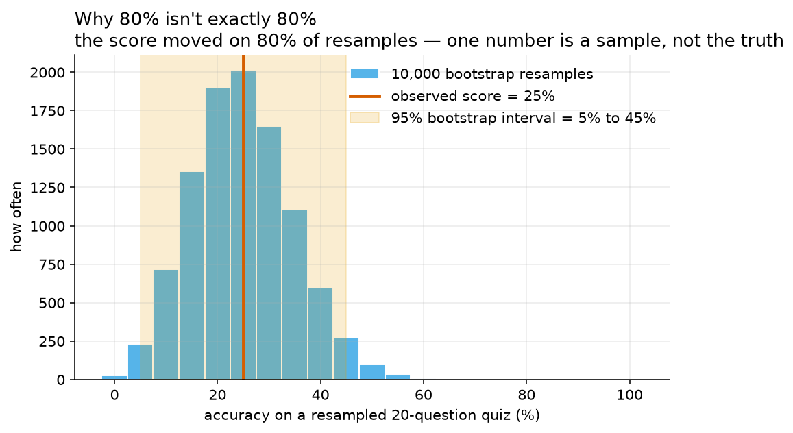
are sky blue and rise in steps of 5 percentage points, from 0 percent to 65 percent, with the tallest bar at 25 percent. A vertical vermillion line marks the observed score of 25 percent. An orange shaded band covers the 95 percent bootstrap interval from 5 percent to 45 percent, and the band is wide, covering most of the histogram. :width: 100%
Every score that ten thousand imitation twenty-question tests produced, built from the model’s
own answers to the real twenty questions. The vertical line is the one score we measured, 25.0
percent. The shaded band is the 95 percent bootstrap interval, 5.0 percent to 45.0 percent. The
band’s width is the honest uncertainty of a twenty-question benchmark. Data from
lab/out/we6_eval.json, seed 20260912.
Read the bars, not the line. The line is where the measurement happened to land. The bars are everywhere it could plausibly have landed instead.
12.6 What resampling cannot fix
Intuition
The bootstrap gave you an interval without a formula, and it never produced an impossible accuracy. That might leave the impression that resampling is a general repair for small samples.
It is not, and the reason is visible in the histogram above. Look at the bars. They are not a smooth hill. They are separated, with gaps between them, like a comb.
Here is why. On a twenty-question test, how many questions can a model get right? It can get 0 right, or 1, or 2, and so on up to 20. There is nothing in between. There is no such thing as getting 7.4 questions right.
So the score can only be , or , or , and so on. Those are 0 percent, 5 percent, 10 percent, 15 percent, and so on. There are only twenty-one scores in existence, and they sit 5 percentage points apart.
That is a property of the test, not of the model and not of your method. No amount of resampling, no cleverness of formula, and no increase in the number of resamples can produce a score of 27 percent on a twenty-question test, because 27 percent is not a thing that can happen.
This is called granularity, or coarseness. It is the reason a reported benchmark score of “87.3 percent” should make you ask how many questions were on the test. If it was twenty questions, 87.3 percent is not a possible answer and somebody has done arithmetic you have not been shown.
The mathematics
Formula 12.8: every score a test of questions can produce
1. In words, with no symbols. A test of a given length can only produce a fixed short list of scores: none right, one right, two right, and so on up to all of them right, each divided by the number of questions. There are one more of these than there are questions, and they are evenly spaced.
2. The formula.
3. Every symbol in it.
| Symbol | How to say it out loud | What it means |
|---|---|---|
| “en” | how many questions are on the test | |
| “zero over n, one over n, two over n” | the score if the model gets none right, one right, two right | |
| “and so on” | the pattern continues in the same way. This mark is called an ellipsis. | |
| “n over n” | the score if the model gets every question right, which is 1, or 100 percent | |
| “n plus one” | how many different scores exist. The plus one is for the score of zero. | |
| “one over n” | the gap between one possible score and the next |
4. How to say the whole thing out loud. “The possible scores are zero over n, one over n, two over n, and so on up to n over n. There are n plus one of them, and they are one over n apart.”
5. Worked, on the real test. .
Step 1, count the possible scores.
Step 2, find the gap between neighbouring scores.
Step 3, convert that gap into percentage points.
percentage points
Step 4, write out the first few and the last few.
Step 5, check against the real bootstrap. Across ten thousand resamples the lab saw 14 distinct scores, running from 0 percent to 65 percent. Fourteen is fewer than twenty-one, which is right: the resamples never happened to produce the very high scores, because a model with five right answers in the hat is unlikely to draw fifteen of them.
6. What going wrong looks like. The plus one catches people. A twenty-question test has twenty-one possible scores, not twenty, because zero right is a score. A quick check: on a one-question test () there are two possible scores, 0 percent and 100 percent, and . The gap is , which is 100 percentage points, and that is correct: on a one-question test there is nothing between complete failure and complete success.
The frequency table below is what those fourteen scores actually looked like. It is produced by the code cell in the next part of this section, which re-runs the lab’s bootstrap with the lab’s seed.
| resampled score | how many of the 10,000 | share |
|---|---|---|
| 0.0% | 25 | 0.25% |
| 5.0% | 231 | 2.31% |
| 10.0% | 719 | 7.19% |
| 15.0% | 1,353 | 13.53% |
| 20.0% | 1,899 | 18.99% |
| 25.0% | 2,014 | 20.14% |
| 30.0% | 1,650 | 16.50% |
| 35.0% | 1,103 | 11.03% |
| 40.0% | 597 | 5.97% |
| 45.0% | 270 | 2.70% |
| 50.0% | 97 | 0.97% |
| 55.0% | 34 | 0.34% |
| 60.0% | 6 | 0.06% |
| 65.0% | 2 | 0.02% |
Three facts come straight off that table, and the third is the one to remember.
The most common resampled score is 25 percent, the one we measured, at 2,014 of 10,000. The bootstrap centres on your measurement.
Nothing above 65 percent ever happened, in ten thousand tries. There were only five correct answers in the hat, and drawing enough of them to reach 70 percent is possible but did not come up.
The resample came out at something other than 25 percent 7,986 times, which is 79.9 percent of the time. Four times out of five, an imitation twenty-question test disagrees with the real one. If you needed one number to explain why a single benchmark score should not be trusted, that is the number.
Python
Counting the distinct values takes one line. Counting how often each one turned up takes a loop inside a loop, written out in full, because a loop you can read is worth more than a clever line you cannot.
distinct_accuracies = numpy.unique(bootstrap_accuracies)     # each different value, once, sorted
print("how many different scores appeared:", len(distinct_accuracies))
print("score  how often  share")

for one_possible_accuracy in distinct_accuracies:            # take each distinct score in turn
    how_many_times = 0                                       # start this score's counter at zero
    for one_resample_accuracy in bootstrap_accuracies:       # look at all 10,000 resamples
        if one_resample_accuracy == one_possible_accuracy:   # is this resample that score?
            how_many_times = how_many_times + 1              # if so, add one to the counter
    print(str(round(one_possible_accuracy * 100, 1)).rjust(5),
          str(how_many_times).rjust(9),
          str(round(100 * how_many_times / 10000, 2)).rjust(6) + "%")
Output:
how many different scores appeared: 14
score  how often  share
  0.0        25   0.25%
  5.0       231   2.31%
 10.0       719   7.19%
 15.0      1353  13.53%
 20.0      1899  18.99%
 25.0      2014  20.14%
 30.0      1650   16.5%
 35.0      1103  11.03%
 40.0       597   5.97%
 45.0       270    2.7%
 50.0        97   0.97%
 55.0        34   0.34%
 60.0         6   0.06%
 65.0         2   0.02%
numpy.unique(...) takes a long list and returns each different value once, sorted from smallest
to largest. len(...) counts them. Fourteen.
The two for loops are worth reading slowly, because a loop inside a loop is the one piece of
programming in this chapter that is genuinely new. The outer loop walks through the fourteen
distinct scores. For each one, the inner loop walks through all ten thousand resamples and adds
one to a counter every time it finds a match. When the inner loop finishes, how_many_times
holds the count for that one score, and the outer loop moves on to the next.
== with two equals signs asks “are these the same?” and gives back True or False. A single
= would try to change the value instead. This is the most common typing mistake in Python and
it is worth knowing before you make it.
.rjust(5) pads a piece of text on the left with spaces until it is 5 characters wide, so the
columns line up. str(...) turns a number into text so it can be padded.
Finally, the number that summarises the chapter.
number_that_missed_25 = 0
for one_resample_accuracy in bootstrap_accuracies:
    if one_resample_accuracy != 0.25:                        # != means "is not equal to"
        number_that_missed_25 = number_that_missed_25 + 1

print("resamples that did not come out at 25.0 percent:", number_that_missed_25)
print("as a share of all 10,000:", round(100 * number_that_missed_25 / 10000, 1), "percent")
Output:
resamples that did not come out at 25.0 percent: 7986
as a share of all 10,000: 79.9 percent
!= is “is not equal to”, the sign from
Toolkit 19, typed on a keyboard that has no
key.
Seventy-nine point nine percent. The score you measured is the single most likely outcome, and it still fails to reappear four times out of five.
12.7 Two runs, same settings, different answers
Intuition
Everything so far has been our own measurement, which is a weak position to argue from. So here is the same phenomenon, in somebody else’s data, recorded by accident.
The material for this course draws on a public teaching repository from UC Berkeley’s Data
Science Modules, ds-modules/Small_Models_SP26, released under a BSD-3-Clause licence. Its
evaluation folder contains a benchmark notebook and the result files from runs of it.
Two of those result files were committed on the same evening, 27 April 2026, about eleven
minutes apart. The file names carry their timestamps: scores_20260427_194044.csv at 19:40:44
and scores_20260427_195142.csv at 19:51:42. Same exam. Same models. Same configuration file.
And the configuration file contains this line:
TEMPERATURE = 0.0 # 0 = deterministic; best for reproducible evalsTemperature 0 means no randomness in the model’s choice of words. It is the setting you use precisely when you want a run to be repeatable. The comment says so.
The two files disagree.
Each file holds 58 rows, one per model per question. Three of those rows differ between the two runs, and all three belong to the same model, Qwen-2.5-7B. Two of the three are short-answer questions graded by another language model acting as a judge, where some wobble is expected.
The third is a multiple-choice question.
On question q1b_iv_A, the earlier run recorded the model’s answer as A, marked wrong, worth
0 of 2 points. The later run recorded the model’s answer as B, marked right, worth 2 of 2
points. The correct answer was B. Multiple choice is scored by exact match, so no judge was
involved. The model’s own answer changed, at temperature 0, eleven minutes apart, on the same
question.
This is not a criticism of the repository. Nobody did anything wrong; a hosted service was called over the internet and it did not return identical output twice. What matters is that the repository committed both files, so the disagreement is on the public record where a student can check it.
Two lessons come out of it, and they are different lessons.
The first is about reproducibility. “Deterministic settings” is a claim about the model, not about the whole pipeline. Everything between you and the model can add variation.
The second is the one that belongs in this chapter. The two headline numbers that came out of those two files differ by more than most published model comparisons.
The mathematics
No new formula. This section uses Formula 12.1, the sample proportion, with one change: the top and bottom are points rather than questions, because the exam awards partial credit on short answers.
Before the arithmetic, work out where the number 58 comes from, because it is a small check you can do on any result file. The exam has 29 questions. Two models sat it. Each row of the file records one model’s answer to one question, so the file should hold
rows
and it does. When a result file’s row count does not match the number of models times the number of questions, something was dropped or duplicated, and you want to know that before you compute anything from it.
Now the scores themselves.
Now hold that 3.9 percentage points next to something. In Chapter 13 you will compare two different models on the same twenty-question bank and find a gap of 25 percentage points that a proper test cannot call significant. Here, a single model compared with itself, eleven minutes apart, moved 3.9 percentage points with no change to anything a person controls.
If a leaderboard separates two models by 2 percentage points, you now know what to ask.
There is one more thing to say, and it is a refusal rather than a calculation.
You might expect this section to end by putting a confidence interval around 0.6809, the way section 12.3 did for 25 percent. It does not, and the reason is worth more than the interval would be.
Formula 12.2 assumes that every item on the test is scored as either right or wrong, and that every item counts the same. Neither is true here. This exam awards partial credit: one of the three rows that changed moved from 0.0 points to 0.33 points out of 1.0, and another moved from 1.5 points to 1.0 out of 2.0. Items carrying different numbers of points are not equally weighted, and an item scored 0.33 is not a yes or a no. Feeding 32.00 and 47 into Formula 12.2 would produce a number, because arithmetic always produces a number, and that number would not mean what the formula says it means.
Section 12.4 showed you a formula returning an answer that cannot exist. This is the other failure mode, and it is more dangerous, because the answer looks fine. A formula used outside its conditions can return something perfectly plausible and perfectly wrong, and nothing in the output will warn you. The only defence is to check the conditions before you compute, every time: is every item scored 0 or 1, does every item count the same, and were the items drawn independently?
So the honest report on these two files is the one the arithmetic above supports: two runs, eleven minutes apart, at temperature 0, differing by 3.9 percentage points on 3 of 58 rows. That statement needs no interval to do its work.
Python
qwen_points_run_one = 32.00        # from scores_20260427_194044.csv
qwen_points_run_two = 33.83        # from scores_20260427_195142.csv
points_available = 47              # the exam total

qwen_score_run_one = qwen_points_run_one / points_available    # Formula 12.1, on points
qwen_score_run_two = qwen_points_run_two / points_available
gap_between_the_runs = qwen_score_run_two - qwen_score_run_one

print("run at 19:40:44:", round(qwen_score_run_one, 4))
print("run at 19:51:42:", round(qwen_score_run_two, 4))
print("gap            :", round(gap_between_the_runs, 4), "which is",
      round(gap_between_the_runs * 100, 1), "percentage points")
Output:
run at 19:40:44: 0.6809
run at 19:51:42: 0.7198
gap            : 0.0389 which is 3.9 percentage points
Three divisions and a subtraction. The arithmetic is the easiest in the chapter and the conclusion is the hardest to argue with, because the data is not ours.
Note what the code does not do. It does not average the two runs into one number. Averaging two runs and reporting the average as “the model’s score” hides exactly the thing you were meant to see. If you have two runs and they disagree, that disagreement is a measurement, and it belongs in the report.
The second cell checks the control, which is the part that makes the first cell mean something. If both models had moved, the sensible conclusion would be that the service was having a bad evening. One model moving and the other not is a different finding.
llama_points_run_one = 27.83       # from scores_20260427_194044.csv
llama_points_run_two = 27.83       # from scores_20260427_195142.csv
llama_score_run_one = llama_points_run_one / points_available
llama_score_run_two = llama_points_run_two / points_available

rows_in_each_file = 58             # two models times 29 questions
rows_that_changed = 3              # all three of them belonged to Qwen-2.5-7B
share_of_rows_that_changed = rows_that_changed / rows_in_each_file

print("Llama run one:", round(llama_score_run_one, 4))
print("Llama run two:", round(llama_score_run_two, 4))
print("did Llama move?", llama_score_run_two != llama_score_run_one)
print("rows that changed:", rows_that_changed, "out of", rows_in_each_file)
print("as a share:", round(share_of_rows_that_changed * 100, 1), "percent")
Output:
Llama run one: 0.5921
Llama run two: 0.5921
did Llama move? False
rows that changed: 3 out of 58
as a share: 5.2 percent
!= is “is not equal to”, and Python answered False: Llama-3.2-3B scored 0.5921 in both runs,
to four decimal places and in fact to every decimal place, because it earned the same 27.83
points twice.
So the two files are identical on 55 of their 58 rows. Five point two percent of the rows moved, and that was enough to move one model’s headline score by 3.9 percentage points while leaving the other model’s score untouched. A small number of rows can carry a large share of a difference, which is the same lesson as section 12.6 arriving from the other direction: with few items, each item is worth a lot.
12.8 How many questions would be enough?
Intuition
Twenty questions gave an interval from 6 percent to 44 percent. That is useless, and you have now seen why from three directions.
The natural question is the practical one. How many questions would it take?
Start from what you want, rather than from what you have. Decide how precise you need the answer to be, and then work backwards to the number of questions that buys that precision. “Precise enough” has to be a number: say you want the score pinned to within 5 percentage points either way, so a model that measures 70 percent is somewhere between 65 percent and 75 percent.
There is one wrinkle, and it is a nice one. The number of questions you need depends on the accuracy, and you do not know the accuracy until you have run the test. The way out is to plan for the worst case. Formula 12.2 told you the standard error is largest when the accuracy is 0.5, so design the test as if the accuracy will be 0.5 and you are safe whatever it turns out to be.
Before the formula, feel the shape of the answer. The standard error has underneath a square root. To halve a square root you must quarter what is inside it. So cutting the interval in half costs you four times as many questions. Getting ten times more precise costs a hundred times as many questions. Precision is expensive, and it gets more expensive the more of it you have. This is why nobody measures anything to arbitrary precision, and why “we ran a bigger benchmark” is a real engineering claim rather than a boast.
The mathematics
Formula 12.9: how many questions a benchmark needs
1. In words, with no symbols. Decide how far you are willing to be wrong. Divide the critical value by that distance, square the result, and multiply by the accuracy times one minus the accuracy. That is how many questions you need. If you do not know the accuracy yet, use one half, which is the worst case and therefore the safe one.
2. The formula.
3. Every symbol in it.
| Symbol | How to say it out loud | What it means |
|---|---|---|
| “en” | the answer: how many questions the test needs | |
| “z star” | the critical value, 1.96 for 95 percent confidence | |
| “aitch” | the half-width you want, as a decimal. Wanting “plus or minus 5 percentage points” means . | |
| the fraction bar | “divided by” | divide by |
| “all squared” | work out the bracket first, then multiply it by itself | |
| “times” | multiply | |
| “p hat times one minus p hat” | the same pair of shares as in Formula 12.2. Use 0.5 for both when you do not know. |
4. How to say the whole thing out loud. “N is z star divided by h, all squared, times p hat times one minus p hat.”
5. Worked, for plus or minus 5 percentage points.
Step 1, write down what you want. , and use the worst case .
Step 2, divide the critical value by the half-width.
Step 3, square that.
Step 4, work out the worst-case share product.
Step 5, multiply.
Step 6, round up to a whole question, because you cannot ask 0.16 of a question.
385 questions
6. What going wrong looks like. Two checks. First, a bigger , meaning you are willing to be less precise, must give a smaller . Try : , squared is 384.16, times 0.25 is 96.04, so 97 questions. Halving the precision demand cut the cost by about four. Second, the answer must be rounded up rather than to the nearest whole number. Rounding 384.16 down to 384 leaves you slightly short of the precision you asked for.
Now run that formula across a range of test sizes and look at the price list.
| questions on the test | half-width at the worst case | the interval around a 70% score |
|---|---|---|
| 20 | plus or minus 21.9 points | 48.1% to 91.9% |
| 100 | plus or minus 9.8 points | 60.2% to 79.8% |
| 200 | plus or minus 6.9 points | 63.1% to 76.9% |
| 384 | plus or minus 5.0 points | 65.0% to 75.0% |
| 1000 | plus or minus 3.1 points | 66.9% to 73.1% |
Both right-hand columns were computed at the worst case, , and not at the 70 percent named in the third heading. That is on purpose. You fix the length of a test before you know what it will score, so you price the widest interval the test could produce. A model that really does land at 70 percent gets a slightly narrower interval than the third column shows, never a wider one. On twenty questions, for instance, Formula 12.2 at gives , then , then , then . That is 20.1 points, not 21.9.
Read the first row and the last row together. Going from 20 questions to 1,000 questions is 50 times the work, and it buys you a seven-fold improvement in precision, from about 22 points to about 3 points. That is the square root, visible as a price.
This is where the published recommendation comes from.
Python
One loop, printing the price list.
print("questions   half width at p = 0.5")

for questions_on_the_test in [20, 100, 200, 384, 1000]:      # the five test sizes to price up
    worst_case_standard_error = math.sqrt(0.5 * 0.5 / questions_on_the_test)   # Formula 12.2
    half_width = 1.96 * worst_case_standard_error                              # Formula 12.3
    print(str(questions_on_the_test).rjust(9), "    plus or minus",
          str(round(half_width * 100, 1)).rjust(4), "points")
Output:
questions   half width at p = 0.5
       20     plus or minus 21.9 points
      100     plus or minus  9.8 points
      200     plus or minus  6.9 points
      384     plus or minus  5.0 points
     1000     plus or minus  3.1 points
for questions_on_the_test in [20, 100, 200, 384, 1000]: loops over a list written out by hand.
Each time round, questions_on_the_test holds the next value from the list. The two lines inside
the loop are Formula 12.2 and then Formula 12.3, applied at the worst case where both shares are
0.5.
Now run it the other way round: name the precision you want, and get the number of questions.
wanted_half_width = 0.05                                     # plus or minus 5 percentage points
questions_needed = (1.96 / wanted_half_width) ** 2 * 0.5 * 0.5

print("z star divided by the half width:", round(1.96 / wanted_half_width, 1))
print("that squared                    :", round((1.96 / wanted_half_width) ** 2, 2))
print("times 0.25                      :", round(questions_needed, 2))
print("rounded up to a whole question  :", math.ceil(questions_needed))
Output:
z star divided by the half width: 39.2
that squared                    : 1536.64
times 0.25                      : 384.16
rounded up to a whole question  : 385
** is Python’s way of writing a power, so x ** 2 means squared. See
Toolkit 5 for what a power is.
math.ceil(...) is the ceiling from Formula 12.6: round up to the next whole number. There is
also round(...), which goes to the nearest, and math.floor(...), which goes down. For
sample size you want ceil, because 384 questions leaves you a fraction short of what you asked
for.
Every number printed there matches a step of the hand arithmetic: 39.2, then 1536.64, then 384.16, then 385.
Common mistakes
Numbered, so you can be told “that is number 4” and know what is meant.
Reporting a score without an interval. “The model scored 25 percent” is not a result. “25 percent, 95 percent interval 6 percent to 44 percent, on 20 questions” is a result. If you report the first one, the reader cannot tell whether your model beats guessing.
Thinking the wobble comes from the model. The model in this chapter is deterministic. Run it a thousand times on these twenty questions and it gives the same five right answers every time. The variability is in which questions got asked, not in the model. People look for the randomness in the wrong place and then conclude, wrongly, that fixing the seed or setting temperature to zero removes the need for an interval.
Trusting the Wald interval near 0 or 1. At 8 right out of 10 it returns an upper end of 104.79 percent. Before using it, check that there are a decent number of right answers and a decent number of wrong answers. Ten of each is the usual rule of thumb. When that fails, use Wilson.
Chopping an impossible interval off at 1. Turning into looks like a fix and is not one. Wilson gives , which is lower at both ends. Trimming the top leaves the bottom wrong.
Confusing percent with percentage points. Moving from 20 percent to 30 percent is a rise of 10 percentage points and also a rise of 50 percent. The standard error of 0.0968 is 9.68 percentage points. Saying “9.68 percent” means something different and usually something false. See Toolkit 11.
Believing more resamples means more certainty. Going from 10,000 resamples to 1,000,000 does not narrow your interval, because it does not add a single question. More resamples only smooth out the simulation’s own noise. The bootstrap cannot overcome a small sample; it can only show you how small it is.
Reporting more digits than the test can produce. A twenty-question test produces scores in steps of 5 percentage points. Writing 25.0 percent is fine; writing 25.03 percent is not, because that number cannot occur. Check that the score you print is one the test can actually give.
Rounding partway through and then reporting extra digits. Round once, at the end. Rounding the standard error to 0.0968 and then reporting the interval to five decimal places claims a precision you threw away two steps earlier.
Averaging two disagreeing runs and reporting the average. If two runs of the same benchmark differ, that difference is a measurement about your pipeline. Report both, then explain. The average hides the finding.
Reading a confidence interval as a probability about the truth. The careful statement is about the procedure: a method that, used repeatedly, captures the true value about 95 times in 100. In practice the useful reading is “values in this range are consistent with what I saw, and values outside it are not”, and that reading will not get you into trouble.
What to remember
A benchmark score is a sample proportion, so it is a quantity that moves when the questions change, not a fixed property of the model. The size of that movement is the standard error, , which was 0.0968 on our twenty-question run and turns into a Wald interval from 6.0 percent to 44.0 percent, or 11.19 percent to 46.87 percent once the Wilson formula repairs it for a count that small. The textbook Wald formula carries assumptions and breaks near 0 and 1, returning an accuracy of 104.79 percent at 8 right out of 10, where Wilson correctly returns 0.4902 to 0.9433. The bootstrap reaches nearly the same answer by resampling instead of by formula, 5.0 percent to 45.0 percent, and it also reveals that a twenty-question test can only produce scores 5 percentage points apart and disagreed with itself on 79.9 percent of resamples. Report the interval, report the number of questions, and if you want a score good to within 3 percentage points, ask 1,068 questions.
Practice problems
Twenty-six problems in three tiers. Warm-up checks that you can do the arithmetic. Practice checks that you can apply it. Stretch checks that you can reason with it.
Worked solutions to the odd-numbered problems are in the Answers appendix. Do the problem before you look.
Unless a problem says otherwise, use and round your final answer to four decimal places or one decimal place as a percentage.
Warm-up
A model answers 12 of 20 questions correctly. Write the accuracy three ways: as a fraction, as a decimal, and as a percentage.
Compute for each of , , and .
Compute for . Then do it for . What do you notice, and can you say why?
Compute and without a calculator if you can, then check both on one.
A model scores 10 out of 20. Compute the standard error, showing all five steps.
The standard error of a score is 0.0671. Compute the margin of error at 95 percent confidence.
A model measures 90 percent accuracy with a margin of error of 0.1315. Write down the two ends of the Wald interval, as decimals and as percentages.
How many different scores can a 25-question test produce? How far apart are they, in percentage points?
Convert 0.0603 to a percentage. Convert 44.0 percent to a decimal. Convert to a percentage.
Which interval is wider, or ? By how many percentage points?
Practice
A model answers 15 of 20 questions correctly. Compute , the standard error, the margin of error, and the 95 percent Wald interval. Show every step.
For that same result, 15 out of 20, compute the Wilson interval. Show all nine steps. Compare the two intervals and say which you would publish.
Compute the plus four interval for 8 out of 10. Compare it with the Wilson interval from Formula 12.4 and say how close the shortcut got.
A five-question test gave the results in question order. You draw the question numbers with replacement. Score that resample by hand.
Using the frequency table in section 12.6, what share of the 10,000 resamples came out at 20 percent or below? Add up the relevant rows and show your working.
Using the same table, what share came out at 40 percent or above?
The two halves of the real twenty-question run scored 20 percent and 30 percent. A colleague asks which of those is the model’s accuracy. Write a three-sentence reply.
Compute the worst-case half-width for a 50-question test. Then use Formula 12.9 to find how many questions you need for a half-width of 10 percentage points.
Using the two Berkeley result files from section 12.7, verify both of Qwen-2.5-7B’s scores from the raw points, and compute the gap in percentage points. Then compute what share of the 58 rows changed.
A model answers 0 of 20 questions correctly. Compute the Wald interval. Describe what the result claims, and say why it cannot be right.
Stretch
Compute the Wilson interval for 0 out of 20. Compare it with your Wald answer from problem 20 and explain, in your own words, what Wilson did differently and why it is the better report.
Compare a test of 100 questions with a test of 400 questions, both at . Compute both margins of error. Show that quadrupling the number of questions halves the margin, and explain which part of Formula 12.2 causes that.
The Wald interval on the real run was and the bootstrap interval was . The bootstrap is wider at both ends. Using Formula 12.8 and the frequency table, explain why a percentile interval on a twenty-question test tends to land on rounder, wider values than the formula does.
A vendor’s website reports that their model “scores 87.3 percent on college-level mathematics”. Write down the three questions you would need answered before you could judge that claim, and say for each one what a bad answer would look like.
Miller recommends at least 1,000 questions. Using Formula 12.9 in reverse, compute the worst-case half-width that 1,000 questions buys. Then compute how many questions would be needed to halve that half-width again, and comment on whether that is a reasonable thing to ask of a benchmark.
Two models sat the same twenty-question bank. One scored 70 percent and the other scored 95 percent. A colleague computes a separate Wald interval for each, notices that the two intervals overlap, and concludes that the models are indistinguishable. Explain why comparing two separate intervals is the wrong analysis for this design, and describe in words what a better analysis would use instead. Chapter 13 does this properly; answer from the idea, not from the formula.