Can a model take a test? - Inside the Machine: The Mathematics of Small Language Models

Chapter 11. Can a model take a test?

What you need before this chapter¶

This is a short and honest list. If any line on it makes you uneasy, follow the link, read that one section of the Math Toolkit, and come back. Nothing on the list takes more than ten minutes.

You will need	Where it is taught from zero
What it means when a letter stands for a number	Toolkit 1, a letter standing for a number
Small numbers written below a letter, like $\hat{p}_1$ and $\hat{p}_2$	Toolkit 2, subscripts
The four ways this book writes “multiply”	Toolkit 3, multiplication
That a fraction bar means “divide the top by the bottom”, and that the sign $\div$ gives the same instruction	Toolkit 4, the fraction bar
Exponents, the small raised number after another number	Toolkit 5, exponents
What a negative exponent such as $e^{-6.163}$ does	Toolkit 6, negative exponents
The number $e$ , and the `exp` key on a calculator	Toolkit 7, the number $e$
What a logarithm answers	Toolkit 8, logarithms
Turning a fraction into a decimal into a percentage	Toolkit 11, percentages and decimals
The difference between a percent and a percentage point	Toolkit 11a, percentage points
What “out of” means	Toolkit 12, proportions
Which way is the x-axis on a bar chart	Toolkit 13, reading a graph
Rounding, and how many decimal places to keep	Toolkit 16, rounding
The signs $>$ and $<$	Toolkit 19, inequalities

You do not need calculus. You do not need to have written code before. You do not need to remember anything about softmax from Chapter 4, although this chapter points back there once, and that pointer is optional.

Setting up¶

Every chapter in this book opens with one block of code that gets the tools ready. Run it once, at the top, and everything later in the chapter will work. Each line has a comment above it saying what that line is for.

# os lets Python read and change settings on your computer. The line under it says
# where the downloaded models are kept, and it MUST come before the transformers imports.
import os
os.environ["HF_HOME"] = r"C:\math3219\models"

# json reads the result files that this course's lab wrote. Every measured number
# in this chapter comes out of one of those files.
import json

# math gives us exp(), which turns a log-probability back into an ordinary probability.
import math

# torch is the numerical library the language model runs on. Only Section 11.3 needs it.
import torch

# AutoTokenizer chops text into the pieces a model understands, and puts them back together.
from transformers import AutoTokenizer

# AutoModelForCausalLM loads the model itself, the pile of learned numbers, from the folder
# it was downloaded into.
from transformers import AutoModelForCausalLM

# matplotlib draws charts.
import matplotlib.pyplot as plt

# The Okabe-Ito colour palette. These colours stay distinguishable for readers with the
# common forms of colour blindness, so this book uses no others.
okabe_ito_blue = "#0072B2"
okabe_ito_orange = "#E69F00"
okabe_ito_green = "#009E73"
okabe_ito_vermillion = "#D55E00"
okabe_ito_purple = "#CC79A7"
okabe_ito_grey = "#999999"

# Chart defaults, so every figure in this chapter looks the same.
plt.rcParams["figure.dpi"] = 140
plt.rcParams["font.size"] = 11
plt.rcParams["axes.spines.top"] = False
plt.rcParams["axes.spines.right"] = False

# The folder holding the lab's result files, relative to the top of the course repository.
results_folder = "lab/out/"

Two notes on that block. The word import means “go and fetch a toolbox somebody else wrote, and make it available to me”. The name after import is the name of that toolbox. A line beginning with # is a comment: Python ignores it completely, and it is there for you.

If you are reading rather than running, skip the block. Every output in this chapter is printed below the code that produced it.

A ninety-five percent that means nothing¶

A tow yard off Chester Avenue in Bakersfield gets an email. A company is selling an artificial intelligence assistant that answers customer phone calls, and the email says the assistant is 95% accurate.

Ask yourself what you would need to know before you believed that.

You would want to know how many questions it was asked. Ninety-five percent of twenty questions and ninety-five percent of twenty thousand questions are not the same claim, and one of them is close to worthless. You would want to know what the questions were, and whether they look anything like the calls a tow yard actually gets at eleven at night. You would want to know what counted as a right answer, and who decided. You would want to know what a machine that knew nothing at all would have scored on the same questions, because on some tests that number is zero and on others it is already 25%.

Here is the uncomfortable part. This course’s own lab produced a 95% as well. A model called Qwen2.5-3B-Instruct answered nineteen out of twenty statistics questions correctly, which is 95.0%, and that number is real, and it is sitting in a file you can open right now. It still does not mean what the email means. It means something narrower and far more useful, and saying exactly what it means is the work of this chapter.

Kern County has a long relationship with tests that carry weight. A commercial driver’s licence, a nursing board exam, a well-control certification out in the oil patch: each one is a fixed set of questions, a fixed pass mark, and a number at the end. Everyone involved understands that the number belongs to the test as much as to the person. Nobody says “she is 87% good at nursing”. They say she scored 87 on that exam, on that day.

Language models get the other treatment. A score gets detached from the test that produced it, printed on a slide, and quoted for a year afterwards. This chapter puts the score back on top of its test. By the end you will be able to take any accuracy claim, including one of your own, and say out loud the four things that have to be attached to it before it means anything at all.

Where every number in this chapter comes from

We never publish a number we did not compute.

Every measured number below was produced by a script in this course’s lab/ folder, running a real model on a documented machine, and written into a file in lab/out/ that you can open.

The main file for this chapter is lab/out/lab4_size_ladder.json, written by lab/lab4_size_ladder.py. It holds the parameter counts, file sizes, scores and timings of three models on one twenty-question bank. The single-question example in Section 11.3 comes from lab/out/appendix_python_reference_checks.json, and it was re-run while this chapter was being written to confirm that the same numbers still come back.

Some examples here use small invented numbers, because 3 out of 4 is easier to check on a phone than 494,032,768. Those are labelled made up for practice. Anything labelled real is what a model actually did.

The question bank holds twenty questions. Twenty is too few to settle a comparison. This chapter says so out loud more than once, and Chapter 12 does the arithmetic that proves it.

Learning objectives¶

By the end of this chapter you will be able to:

(Understand) Explain what a proportion is, and convert between a proportion, a decimal and a percentage in both directions, without a calculator in simple cases.
(Apply) Compute a model’s accuracy on a bank of questions as a sample proportion $\hat{p} = x / n$ , and report it with its denominator attached.
(Analyze) Work out the chance level of a multiple-choice test from the number of options, and judge whether a measured score is meaningfully above it.
(Apply) Describe how an answer is pulled out of a model by ranking the log-probabilities of the option letters, and explain why that is a decision you make rather than a reading you take.
(Analyze) Read a controlled experiment in which three models of different sizes sit one bank under one procedure, name what was held constant, and state what the result does and does not license you to claim.

This lesson at a glance¶

A score is a proportion: the number right divided by the number asked, which is a number between 0 and 1 that you can also write as a percentage.
Chance is the floor: on a question with four options, a machine that knows nothing scores 25%, so 25% is the number a real score has to beat.
An answer has to be extracted: the model produces a spread of scores across its whole vocabulary, and turning that into “the model said B” is a procedure somebody chose.
One variable at a time: three models, one family, one bank, one procedure, and the parameter count is the only thing allowed to move.

The vocabulary of this chapter¶

Every term below appears later in the chapter. They are collected here, before they are used, so that no sentence in this chapter contains a word you have not been given.

Term	What it means, in one line
Benchmark	A fixed set of questions with known right answers, used to score a model.
Question bank	The actual collection of questions in a benchmark. Ours holds twenty.
Item	One question in the bank, with its options and its known right answer.
$n$	How many questions were asked. Said “en”. For us, $n = 20$ .
$x$	How many questions the model got right. Said “ex”. A whole number.
Proportion	A part divided by a whole. Always between 0 and 1.
Fraction	One number written above another with a bar between them, such as $\frac{3}{20}$ . The bar means “divide”.
Decimal	A number written with a point in it, such as 0.15. A proportion is usually written as a decimal.
Percentage	A proportion multiplied by 100, with a `%` sign after it. 0.15 is 15%.
Percentage point	The unit for the gap between two percentages. 70% minus 15% is 55 percentage points.
Accuracy	The proportion of questions a model answered correctly.
Sample proportion, $\hat{p}$	A proportion measured on a sample rather than on everything. Said “p-hat”.
Chance level	The score a machine that knows nothing would get by guessing.
Expected number	A long-run average over many runs, not a prediction about any one run.
Answer extraction	The procedure that turns what the model produced into “the model said B”.
Token	One of the fixed pieces of text a model works in. Our models know 151,936 of them. Chapter 2 builds them from zero.
Tokenizer	The tool that chops text into tokens, and puts tokens back together into text.
Softmax	The step that turns a model’s raw scores into probabilities that add to 1. It is all of Chapter 4, and this chapter needs only one fact about it.
Log-probability	The natural logarithm of a probability. Always a negative number.
Argmax	“The position of the largest one.” It hands back a position, not a value.
Forward pass	One run of the model over one piece of text. The unit of work, and of cost.
Parameter	One number inside the model, learned during training and fixed afterwards. Chapter 3 takes them apart.
Ratio	One number divided by another, kept as a bare number. “Three times as many” is a ratio of 3.
Byte	Eight bits of computer storage. A bit is a single yes-or-no.
FP16	A way of storing one number in 16 bits, which is 2 bytes. Chapter 6 is about what that costs you.
Gigabyte, GB	One billion bytes, on the plain decimal counting this book uses.
Controlled experiment	A comparison in which everything is held still except the one thing being studied.
Variable	Anything in an experiment that could have taken a different value.
Confound	A second variable that moved when it should not have, so you cannot tell which one caused the result.
Model family	A group of models trained the same way by the same people, differing mainly in size.
Naive scoring	The first scoring procedure anyone reaches for. Ours ranks the letters A, B, C and D.
Rotation	Sliding a list of options along by one position, with the last one wrapping around to the front.
Rotation-debiased scoring	A repaired procedure that asks each question several times with the options in different orders.
Consistency	How many questions on which shuffling the options made no difference to whether the model got them right.
Standard error	A measure of how far a measured score would bounce around if you asked a different set of questions. Chapter 12 builds it from zero.
Margin of error	How far either side of a measured score the true value could reasonably sit. Written with a ± sign, said “plus or minus”.
Paired	Two scores are paired when both models answered the same questions, so the two lists of results line up question by question.

Two of those, naive scoring and rotation-debiased scoring, are named here because the result file names them, and because you are going to see two columns of numbers rather than one. This chapter does not take those procedures apart. Chapter 13 does, and taking them apart is the whole of Chapter 13.

11.1 A score is a proportion¶

Intuition¶

Think about the last time somebody told you a score. “I got eighteen.” Your very next question was almost certainly “out of what?”, and you asked it without thinking, because eighteen on its own is not information. Eighteen out of twenty is excellent. Eighteen out of a hundred is a disaster. The number eighteen did not change. What changed is the thing it was measured against.

That second number has a name. It is the whole, or the total, or in the notation this book uses, $n$ . And the operation that welds the two numbers into one meaningful quantity is division. Eighteen out of twenty means eighteen divided by twenty.

When you do that division you get 0.9. That number, 0.9, is a proportion. A proportion answers the question “what share of the total is this?” and it always lands somewhere between 0 and 1. Zero means none of them. One means all of them. Nothing else is possible, which is the first and most useful sanity check in this entire chapter.

People often find proportions slippery because the same quantity gets written three different ways and nobody says that they are the same quantity. Here are the three ways, side by side, for eighteen out of twenty.

As a fraction: $\frac{18}{20}$ . This is the raw record of what happened. Eighteen, out of twenty. The line between the two numbers is a fraction bar, and it is an instruction to divide the top number by the bottom one. See Toolkit 4.
As a decimal: 0.9. This is what you get when you actually carry out the division.
As a percentage: 90%. This is the decimal multiplied by 100, with a percent sign glued on the end.

Those are not three different answers. They are one answer wearing three coats. Getting comfortable moving between them is most of what “doing the maths” means in this chapter, and it is worth more to you than any formula in the book.

Now the point that makes this a chapter about language models rather than a chapter about fractions. When a model sits a test, its score is a proportion. The part is how many questions it got right. The whole is how many you asked. That is the entire definition of accuracy. It is not a mysterious property of the model. It is a division you can do by hand.

The mathematics¶

Two formulas live in this section. The first turns counts into a proportion. The second turns a proportion into a percentage. Both are presented the way every formula in this book is presented: in plain words first, then the symbols, then how to say the whole thing out loud, then worked arithmetic with nothing skipped, then a way to check yourself.

Formula 11.1: accuracy as a sample proportion¶

1. In words. Count how many questions the model got right. Divide that count by how many questions you asked. The answer is the model’s accuracy.

2. The formula.

\hat{p} \;=\; \frac{x}{n}

3. The symbols. Every symbol in that line has a row, including the ones you are sure you already know.

Symbol	How to say it out loud	What it means
$\hat{p}$	“p hat”	the answer: the accuracy, a number between 0 and 1
the hat, $\hat{\phantom{p}}$	“hat”	a small mark that says “this number was measured, not known for certain”. It is the difference between “what this model scored on these twenty questions” and “how good this model really is”. Chapter 12 is built on that difference.
$p$	“pee”	short for proportion. The letter is a habit, not a rule; a different book might use $a$ for accuracy. See Toolkit 1.
$=$	“equals”	the thing on the left and the thing on the right are the same number
$x$	“ex”	how many questions the model answered correctly. A count, so a whole number, and never negative.
the fraction bar	“divided by”	divide the number on top by the number underneath. See Toolkit 4.
$\div$	“divided by”	the same instruction as the fraction bar, written along one line instead of stacked. $\frac{3}{20}$ and $3 \div 20$ are the same sum. This book uses whichever one fits the sentence, and the worked examples below use $\div$ because that is the key on a calculator.
$n$	“en”	how many questions were asked. A whole number, and never zero, because dividing by zero is not a thing you can do.

4. Out loud. “P hat equals x over n.” In full English: “the measured accuracy is the number of questions answered correctly, divided by the number of questions asked.”

5. Worked, with real numbers. Qwen2.5-0.5B-Instruct was counted correct on 3 of the 20 questions in this course’s bank under the rotation-debiased procedure. This is real, from lab/out/lab4_size_ladder.json, where it is stored as "rotation_accuracy": 0.15. That procedure asks each question several times with the options in different orders and counts the question correct only if the model finds the right option most of those times. Section 11.6 sets it out in full. For now all you need is the count: 3.

Step 1. Write down the two counts.

x = 3 \qquad n = 20

Step 2. Do the division. On a phone calculator: 3, then the divide key, then 20, then equals.

\hat{p} = 3 \div 20 = 0.15

If long division by hand feels safer, the same result comes from noticing that $20 \times 0.1 = 2$ and $20 \times 0.05 = 1$ , so $20 \times 0.15 = 3$ . Multiplication checking division is a habit worth keeping.

Worked again, for the largest model. Qwen2.5-3B-Instruct was counted correct on 19 of the same 20 questions, under the same procedure (real, same file, "rotation_accuracy": 0.95).

Step 1. $x = 19$ , $n = 20$ .

Step 2. $19 \div 20 = 0.95$ .

Check by multiplying back: $20 \times 0.95 = 19$ . Correct.

6. Check it. Your answer must land between 0 and 1. If you get a number bigger than 1, you divided the wrong way round: you computed $n \div x$ instead of $x \div n$ . Try it and see. $20 \div 3 = 6.667$ to three decimal places, and the digit 6 repeats forever after that. That is not a share of anything, because a model cannot get six and two-thirds times more questions right than you asked. A negative answer is not possible either, since both counts are counts.

Formula 11.2: a proportion written as a percentage¶

1. In words. Take the proportion you computed and multiply it by one hundred. The result is the same quantity expressed as a percentage, which is a share out of a hundred instead of a share out of one.

2. The formula.

P \;=\; \hat{p} \times 100

3. The symbols.

Symbol	How to say it out loud	What it means
$P$	“big pee”	the answer: the same accuracy written as a percentage. We use a capital letter so it is not confused with $\hat{p}$ .
$=$	“equals”	both sides are the same number
$\hat{p}$	“p hat”	the proportion from Formula 11.1, a number between 0 and 1
$\times$	“times”	multiply. The same instruction can be written $\hat{p} \cdot 100$ , or $100\hat{p}$ with no sign at all. See Toolkit 3.
100	“one hundred”	a fixed number. It is 100 because “per cent” is Latin for “per hundred”. See Toolkit 11.
$\%$	“percent”	a sign written after the answer to say which of the two forms you are holding. 0.15 and 15% are the same quantity; the sign is what tells the reader which one is on the page.

4. Out loud. “Big P equals p hat times one hundred.” In full English: “the percentage is the proportion multiplied by a hundred.”

5. Worked, with real numbers. All three are real, from lab/out/lab4_size_ladder.json.

For the smallest model, $\hat{p} = 0.15$ .

P = 0.15 \times 100 = 15.0

so the accuracy is 15.0%.

For the middle model, $\hat{p} = 0.7$ .

P = 0.7 \times 100 = 70.0

so the accuracy is 70.0%.

For the largest model, $\hat{p} = 0.95$ .

P = 0.95 \times 100 = 95.0

so the accuracy is 95.0%.

Multiplying by 100 moves the decimal point two places to the right. 0.15 becomes 15.0 because the point hops over the 1 and then over the 5. Going the other way, from a percentage back to a proportion, you divide by 100, which moves the point two places left: 95.0 becomes 0.95.

6. Check it. A percentage from an accuracy must land between 0% and 100%. If you get 1500% you multiplied by 100 twice. If you get 0.15% you multiplied by 100 zero times and then wrote a percent sign anyway, which is one of the most common slips in this whole subject. Say the number out loud with its unit and the error usually announces itself: “zero point one five percent” should sound wrong for a model that got three questions out of twenty.

Formula 11.2a: how much bigger one score is than another, as a percentage¶

1. In words. Sometimes you want to say how much bigger one number is than another, measured against the smaller one. Divide the new number by the old number. Multiply by one hundred, which tells you what percentage of the old number the new number is. Then take away the hundred percent you already had at the start. What is left over is the increase.

That last subtraction is the step people drop, and dropping it is why this formula gets its own entry.

2. The formula.

g \;=\; \left( \frac{P_2}{P_1} \times 100 \right) - 100

3. The symbols.

Symbol	How to say it out loud	What it means
$g$	“gee”	the answer: the increase, written as a percentage of the starting value. A percent, never a percentage point.
$=$	“equals”	both sides are the same number
the big round brackets, $(\ )$	“bracket”, “close bracket”	do everything inside them before you do anything outside them. Here: divide and multiply first, subtract last.
$P_1$	“big P sub one”	the starting value, the one you are measuring against. Never zero, because you cannot divide by zero.
$P_2$	“big P sub two”	the new value
the subscripts $_1$ and $_2$	“sub one”, “sub two”	labels saying which value is which. See Toolkit 2.
the fraction bar	“divided by”	divide the top by the bottom
$\times$	“times”	multiply
100	“one hundred”	appears twice, doing two different jobs. The first turns a ratio into a percentage. The second is the 100% you started with, which is being taken away.
$-$	“minus”	subtract the thing on the right from the thing on the left

4. Out loud. “G equals, bracket, big P sub two over big P sub one, times one hundred, close bracket, minus one hundred.” In full English: “the increase is the new value written as a percentage of the old value, less the hundred percent you already had.”

5. Worked, with real numbers. The smallest model scored 15.0% and the middle model scored 70.0% (real, from lab/out/lab4_size_ladder.json).

Step 1. Write down the two values. $P_1 = 15.0$ and $P_2 = 70.0$ .

Step 2. Do the division inside the brackets first.

70.0 \div 15.0 = 4.6667

to four decimal places. The digit 6 repeats forever, so this is a place to keep your working long and round at the end. See Toolkit 16.

Step 3. Still inside the brackets, multiply by one hundred.

4.6667 \times 100 = 466.67

The middle model’s score is 466.7% of the smallest model’s score.

Step 4. Now leave the brackets and subtract the hundred percent you started with.

466.67 - 100 = 366.67

which to one decimal place is 366.7%. The middle model scored 366.7% more than the smallest.

Worked again, for the second step of the ladder. $P_1 = 70.0$ and $P_2 = 95.0$ (real, same file).

Step 1. $95.0 \div 70.0 = 1.3571$ to four decimal places.

Step 2. $1.3571 \times 100 = 135.71$ .

Step 3. $135.71 - 100 = 35.71$ , which is 35.7% more.

6. Check it. Two checks, and the second one catches almost everything.

If the new value is larger than the old one, $g$ must be positive. If the new value is smaller, $g$ must be negative, and a negative $g$ is an honest answer that should be reported as one.

If you forget Step 4 you will report 466.7% where you meant 366.7%. Say it out loud and it collapses: “the middle model scored 466.7% more than the smallest” would mean it scored 15.0% plus 466.7% of 15.0%, which is 85.0%, and it did not. It scored 70.0%. The subtraction is not optional.

Last, note the unit. $g$ is a percent. The gap in Definition 11.5 below is in percentage points. The two numbers describe the same pair of scores and they are not interchangeable.

One more thing belongs in this section, because it causes more confusion than any other piece of notation in the course.

Definition 11.5: Percentage point

A percentage point is the unit you use when you subtract one percentage from another.

The smallest model scored 15.0% and the middle model scored 70.0%. The gap between them is $70.0 - 15.0 = 55.0$ percentage points. It is not “55 percent”, because 55 percent would suggest a share of something, and this is a gap between two shares.

Keeping the two words apart lets you say something precise that is otherwise impossible. Going from 15.0% to 70.0% is a gain of 55.0 percentage points. It is also a gain of 366.7% in relative terms, which is Formula 11.2a: $70.0 \div 15.0 = 4.6667$ , then $4.6667 \times 100 = 466.67$ , then $466.67 - 100 = 366.67$ , which is 366.7%. Both statements are true. They are different statements, in different units. Advertising prefers the second one.

See Toolkit 11a.

Python¶

The code below turns counts into proportions and then into percentages. It does not need a model or a graphics card. It needs nothing beyond the arithmetic you did by hand a moment ago, and its purpose is to let you see that Python is doing exactly that arithmetic and nothing cleverer.

# How many questions were on the bank, and how many the smallest model got right.
# Both counts are real, from lab/out/lab4_size_ladder.json.
number_of_questions = 20
number_correct = 3

# Formula 11.1: the proportion is the part divided by the whole.
# The slash / is Python's division sign.
accuracy_proportion = number_correct / number_of_questions

# Formula 11.2: the percentage is the proportion multiplied by one hundred.
# The asterisk * is Python's multiplication sign.
accuracy_percentage = accuracy_proportion * 100

# print() writes things to the screen. Anything inside quotation marks is printed
# exactly as typed; anything without quotation marks is a value we worked out above.
print("questions asked          :", number_of_questions)
print("questions correct        :", number_correct)
print("accuracy, as a proportion:", accuracy_proportion)
print("accuracy, as a percentage:", accuracy_percentage, "percent")

Output:

questions asked          : 20
questions correct        : 3
accuracy, as a proportion: 0.15
accuracy, as a percentage: 15.0 percent

Read that output one line at a time. The first two lines are the numbers that went in. The third line is $3 \div 20$ , which is 0.15, matching the hand arithmetic above exactly. The fourth line is $0.15 \times 100$ , which is 15.0.

Notice that Python printed 15.0 and not 15. The trailing .0 is Python telling you that this is a number that is allowed to have a decimal part, even though on this occasion the decimal part happens to be nothing. It is not an error and it is not extra precision. It is a label on the kind of number.

Now the same arithmetic for all three models. The block below uses a for loop, which is Python’s way of saying “do the following once for each thing in this list”.

# The three correct-answer counts, in order from smallest model to largest.
# All three are real, from lab/out/lab4_size_ladder.json.
count_list = [3, 14, 19]
name_list = ["Qwen2.5-0.5B", "Qwen2.5-1.5B", "Qwen2.5-3B"]

# range(3) produces the positions 0, 1 and 2. Python counts positions from 0,
# so position 0 is the first thing in the list.
for model_position in range(3):
    one_count = count_list[model_position]
    one_proportion = one_count / number_of_questions
    one_percentage = one_proportion * 100
    print(name_list[model_position], one_count, "of", number_of_questions,
          "=", one_proportion, "=", one_percentage, "percent")

Output:

Qwen2.5-0.5B 3 of 20 = 0.15 = 15.0 percent
Qwen2.5-1.5B 14 of 20 = 0.7 = 70.0 percent
Qwen2.5-3B 19 of 20 = 0.95 = 95.0 percent

The square brackets in count_list[model_position] mean “reach into the list and take the item at this position”. The indented lines under the for are the body of the loop: they run three times, once with model_position set to 0, once with it set to 1, and once with it set to 2.

Look at the middle row. Python printed 0.7, not 0.70. Python drops a trailing zero after the point because 0.7 and 0.70 are the same number. When you write this up for a human reader you put the zero back, because 70.0% and 70% read differently to a person even though they are the same to a machine. Toolkit 16 has the rule this book follows for decimal places.

Try it 11.1: from a count to a percentage and back

(a) A model answers 13 of 20 questions correctly. Write its accuracy as a fraction, as a decimal, and as a percentage.

(b) Another model is reported at 45%. On a 20-question bank, how many questions did it get right?

(c) Someone reports an accuracy of 1.35. What went wrong?

11.2 The number a score has to beat¶

Intuition¶

Put a pigeon in front of a four-option multiple-choice test and let it peck at random. It knows nothing about statistics. It cannot read. Over twenty questions it will still get some of them right, because one option in every four is correct and the pigeon keeps landing on options.

How many? On average, a quarter of them. Five out of twenty.

Here is why it is exactly a quarter. Four options are offered and the pigeon has no reason to prefer any of them, so over a long run it lands on each one about equally often. Put it in front of 100 questions and it picks A about 25 times, B about 25 times, C about 25 times and D about 25 times. Exactly one of the four is correct on each question, so the pecks that landed on the correct option number about 25 out of the 100. That is 25 out of 100, which is a quarter, which is 25%. The count of options is the only thing that entered that argument, which is why the chance level depends on nothing else.

That number has a name. It is the chance level, and it is the single most important number to have in your head before you look at any multiple-choice score, because it is the score that corresponds to knowing nothing at all. A model that scores below the chance level has not merely failed; something odd is going on, and you should go and find out what. A model that scores at the chance level has shown nothing. A model that scores above the chance level has done something, and how much something is the question.

Here is why this matters more for language models than for people. A student who guesses on a multiple-choice exam guesses roughly evenly, because they have no reason to prefer one letter over another. A language model has reasons. It has read an enormous quantity of text, including enormous quantities of multiple-choice questions, and it arrives with opinions about letters that have nothing to do with the question in front of it. So a language model’s “guessing” is not necessarily even, and its score can land below chance as easily as above. You will see exactly that happen later in this chapter.

There is one more thing chance level does for you, and it is the thing that keeps people honest. It sets the size of the room. On a four-option test, the whole interesting range runs from 25% to 100%, which is 75 percentage points wide, not 100. So a jump from 25% to 50% is not “half as good as perfect”. Work it out: 50 minus 25 is 25 percentage points of climbing, out of the 75 percentage points the room has in it, and $25 \div 75 = 0.3333$ to four decimal places, which is one third of the way up from the floor. That 3 repeats forever, which is why the answer is written to a stated number of places; see Toolkit 16. Chance level is the floor, and knowing where the floor is stops you from admiring a model for standing on it.

The mathematics¶

Two formulas turn the pigeon argument into numbers. The first works out the chance level from the number of options. The second turns that chance level into a count of questions, which is the form people find easiest to picture. Both are short, and both are presented in the same six parts as every other formula in this book.

Formula 11.3: chance level on a multiple-choice question¶

1. In words. If every question offers the same number of options and only one option is correct, then a guesser picking at random gets one question right for every however-many options there are. Divide one by the number of options.

2. The formula.

c \;=\; \frac{1}{k}

3. The symbols.

Symbol	How to say it out loud	What it means
$c$	“see”	the answer: the chance level, a proportion between 0 and 1
$=$	“equals”	both sides are the same number
1	“one”	the number of options that are correct. One, because exactly one option per question is right.
the fraction bar	“divided by”	divide the top by the bottom
$k$	“kay”	how many options each question offers. For our bank, $k = 4$ . A whole number, at least 2.

4. Out loud. “C equals one over k.” In full English: “the chance level is one divided by the number of options.”

5. Worked, for our bank. Our twenty questions each offer four options, labelled A, B, C and D (real; the bank is printed in full in The Shelf).

Step 1. Write down $k$ .

k = 4

Step 2. Divide.

c = 1 \div 4 = 0.25

Step 3. Turn it into a percentage using Formula 11.2.

P = 0.25 \times 100 = 25.0\%

Worked again, for other option counts, so the pattern is visible. These are made up for practice; no test in this course uses them.

A true-or-false test has two options. $c = 1 \div 2 = 0.5$ , which is 50.0%.

A five-option test has five. $c = 1 \div 5 = 0.2$ , which is 20.0%.

A ten-option test has ten. $c = 1 \div 10 = 0.1$ , which is 10.0%.

The pattern is worth saying out loud: more options means a lower floor, because guessing gets harder as the number of wrong answers grows.

6. Check it. The chance level must be between 0 and 1, and it must be smaller than 1 whenever there are two or more options. If you compute a chance level of 4, you divided $k \div 1$ instead of $1 \div k$ . If your model’s measured accuracy comes out below $c$ by a wide margin, do not congratulate yourself on a hard test. Go and check the scoring procedure, because a machine performing reliably worse than random is a machine that is being read wrongly, and that is a real event you will meet in Section 11.5.

Formula 11.4: how many questions a guesser gets right¶

1. In words. Multiply the number of questions on the test by the chance level. That tells you how many questions a guesser would get right on an average run.

2. The formula.

E \;=\; n \times c

3. The symbols.

Symbol	How to say it out loud	What it means
$E$	“ee”	the answer: the expected number of questions a guesser gets right. “Expected” here is a technical word meaning the long-run average, not a prediction about any one run.
$=$	“equals”	both sides are the same number
$n$	“en”	how many questions are on the test
$\times$	“times”	multiply
$c$	“see”	the chance level from Formula 11.3

4. Out loud. “E equals n times c.” In full English: “the number of questions a guesser gets right is the number of questions multiplied by the chance level.”

5. Worked, for our bank.

Step 1. Write down the two numbers. $n = 20$ and $c = 0.25$ .

Step 2. Multiply.

E = 20 \times 0.25 = 5

A guesser gets 5 of our 20 questions right, on average.

Worked again, on a bigger bank, to show what the formula is good for. This one is made up for practice. Suppose you built a bank of 1,000 four-option questions, which is roughly the size that the research literature recommends and which Chapter 12 explains.

E = 1000 \times 0.25 = 250

A guesser gets about 250 of them. Notice that the proportion did not change at all; it is still 25%. What changed is how tightly a real run clusters around it, and that is the subject of the next chapter.

6. Check it. $E$ must be between 0 and $n$ . If you get a number larger than the number of questions, you multiplied by the percentage 25 instead of by the proportion 0.25, which would give $20 \times 25 = 500$ questions right out of 20. Say that out loud and the mistake announces itself. This is the most common arithmetic slip in the chapter, and the cure is always the same: percentages go back to proportions before they go into a formula.

Now put the two numbers next to each other, because this is where the chapter turns.

The chance level on our bank is 25.0%. A guesser gets about 5 of 20.

Qwen2.5-0.5B-Instruct, scored by the first procedure anyone reaches for, got 5 of 20, which is 25.0% (real, from lab/out/we6_eval.json, where it is stored as "correct": 5 and "accuracy": 0.25).

Those are the same number. A half-billion-parameter language model, trained on an amount of text no person could read in a thousand lifetimes, scored precisely what a pigeon would score.

That coincidence is not a joke and it is not an accident. It is a clue, and following it is Chapter 13, which is the most original piece of work in this course. For now, notice only what the chance level bought you: without it, 25% looks like a low but real score. With it, 25% looks like no score at all, and you know to be suspicious.

Python¶

The block below is Formula 11.3 and Formula 11.4 typed out, in the same order you did them by hand. It carries on from the block in Section 11.1, so the name number_of_questions is already set to 20 and does not need setting again. Read each line, then check the printed answer against the arithmetic you did a page ago.

# Our bank offers four options on every question, labelled A, B, C and D.
number_of_options = 4

# Formula 11.3: the chance level is one divided by the number of options.
chance_proportion = 1 / number_of_options

# Formula 11.2 again: the same quantity as a percentage.
chance_percentage = chance_proportion * 100

# Formula 11.4: how many of our twenty questions a guesser gets right on average.
expected_correct_by_guessing = number_of_questions * chance_proportion

print("options per question           :", number_of_options)
print("chance, as a proportion        :", chance_proportion)
print("chance, as a percentage        :", chance_percentage, "percent")
print("questions a guesser gets right :", expected_correct_by_guessing, "out of", number_of_questions)

Output:

options per question           : 4
chance, as a proportion        : 0.25
chance, as a percentage        : 25.0 percent
questions a guesser gets right : 5.0 out of 20

Four lines of arithmetic, and all four match what you did by hand. 1 / 4 gives 0.25, and 0.25 * 100 gives 25.0, and 20 * 0.25 gives 5.0.

That last one prints as 5.0 rather than 5 for the reason given in Section 11.1: one of the numbers going in had a decimal point in it, so Python keeps the decimal point on the way out. The model did not get five point zero questions right. It got five.

The value number_of_questions was set back in Section 11.1 and is still sitting there. This is what “all the code runs top to bottom in one place” means in practice. If you skipped the earlier block, Python will stop and tell you it does not know what number_of_questions is, and it will be right.

Now try a small table of chance levels, so you can see the floor drop as the number of options rises.

# A list of option counts to look at. Four is ours; the others are for comparison.
option_count_list = [2, 3, 4, 5, 10]

for option_position in range(5):
    one_option_count = option_count_list[option_position]
    one_chance_proportion = 1 / one_option_count
    one_chance_percentage = one_chance_proportion * 100
    # round() cuts a number down to a given number of decimal places, so the
    # column stays readable. It changes what is printed, not what is stored.
    print(one_option_count, "options ->  chance =", round(one_chance_percentage, 1), "percent")

Output:

2 options ->  chance = 50.0 percent
3 options ->  chance = 33.3 percent
4 options ->  chance = 25.0 percent
5 options ->  chance = 20.0 percent
10 options ->  chance = 10.0 percent

Check that table before you use it. Every line in it is a division you can do in your head: $1 \div 2$ is a half, $1 \div 4$ is a quarter, $1 \div 10$ is a tenth. If one of those lines had come out wrong, you would want to notice, and the only way to notice is to have done the arithmetic yourself first. Every table in every paper you will ever read was printed by somebody’s loop, and loops have bugs in them.

The third row, 33.3, is the one to look at twice. One divided by three does not stop. The digits go 0.333333 and keep going forever. The round(one_chance_percentage, 1) in the code cut it to one decimal place for printing, which is why the column lines up. The number stored inside Python is still the long one. Rounding for display and rounding in a calculation are different acts, and mixing them up is how small errors get into big tables.

Try it 11.2: the floor of the room

(a) A benchmark uses questions with three options each. What is the chance level, as a proportion and as a percentage?

(b) On that three-option benchmark with 60 questions, how many does a guesser get right on average?

(c) Model A scores 40% on a four-option test. Model B scores 40% on a ten-option test. Which result is more impressive, and why?

11.3 Getting an answer out of a model¶

Intuition¶

Marking a paper exam is easy in one specific way: the student wrote “B” in a box, and B is what they meant. There is a mark on the page. You read it.

A language model does not write a mark on a page. What it produces, every single time, is a score for every possible next piece of text. Not one answer. A score for all of them. For the models in this course there are 151,936 possible pieces, called tokens, which is the subject of Chapter 2. The commas in that number are there to break the digits into groups of three so the eye can count them. They are not decimal points and they do not change the value: the number is one hundred and fifty-one thousand, nine hundred and thirty-six. See Toolkit 17.

The model hands you 151,936 numbers, and somewhere in that list are the numbers for “A”, “B”, “C” and “D”, and also the numbers for “the”, “Paris”, a blank space, a line break, and a symbol used in written Japanese.

So there is no mark on the page to read. Somebody has to decide which of those 151,936 numbers counts as the model’s answer. That decision has a name: answer extraction. And here is the sentence that this whole section exists to deliver:

Answer extraction is a decision you make, not a reading you take.

Once you see that, you cannot unsee it, and a great deal of published AI evaluation starts to look different.

There is one approach that almost everybody reaches for first, and it is the one this course’s lab used first too. Write the question out with its four options, end the text with the word Answer: and nothing after it, and then ask the model one narrow question: of the four tokens “A”, “B”, “C” and “D”, which one do you think is most likely to come next? Everything else in the vocabulary is ignored. The four numbers are compared, the biggest wins, and that letter is recorded as the model’s answer.

That approach has real virtues. It gives the same answer every time you run it, with no randomness anywhere, which means your experiment is repeatable. It never has to parse a sentence like “I think the answer is probably B, although C is also defensible.” It is cheap: one run of the model per question.

It also has a flaw, and the flaw is large enough that this course spends a whole week on it. For now, one sentence: the four letters are competing with everything else the model might say, and a model can have opinions about letters that have nothing to do with the question. Hold that thought. Chapter 13 picks it up.

The mathematics¶

Formula 11.5: the extracted answer¶

1. In words. Look at the four numbers the model gave to the four option letters. Find the biggest one. The letter sitting in that position is the model’s answer.

2. The formula.

\hat{a} \;=\; \underset{i \,\in\, \{1,\,2,\,3,\,4\}}{\arg\max}\ \ell_i

3. The symbols. This formula has more furniture than the earlier ones, so every piece of the furniture gets a row too.

Symbol	How to say it out loud	What it means
$\hat{a}$	“a hat”	the answer: which option position the model picked. A whole number from 1 to 4, which you then translate into A, B, C or D.
the hat	“hat”	the same mark as in $\hat{p}$ : this was measured, not known.
$=$	“equals”	both sides are the same thing
$\arg\max$	“arg max”	“the position of the largest one”. It hands back a position, not a value.
$\ell$	“ell”	a script letter L, standing for the log-probability. A different book might write $s$ for score.
$\ell_i$	“ell sub i”	the log-probability the model gave to option number $i$ . The small $i$ underneath is a subscript; see Toolkit 2.
$i$	“eye”	a counter that stands for “whichever option we are looking at”. $i = 1$ means option A, $i = 2$ means option B, and so on.
$\in$	“in”, or “is a member of”	says which values the counter is allowed to take
$\{1, 2, 3, 4\}$	“the set one, two, three, four”	curly brackets hold a set, which is a collection of allowed values. Here the four option positions.
the space before $\ell_i$	nothing	it separates the instruction from the thing the instruction acts on

4. Out loud. “A hat is the arg max, over i in the set one to four, of ell sub i.” In full English: “the model’s answer is whichever of the four options was given the largest log-probability.”

5. Worked, with real numbers. These four numbers are real. They come from lab/out/appendix_python_reference_checks.json, and they were produced by Qwen2.5-0.5B-Instruct on the first question of this course’s bank:

Question: The mean of 2, 4, 4, 6 is: A. 3 B. 4 C. 5 D. 6 Answer:

The four log-probabilities came back as:

\ell_1 = -6.163 \qquad \ell_2 = -7.647 \qquad \ell_3 = -8.4651 \qquad \ell_4 = -8.8911

Step 1. Compare $\ell_1$ and $\ell_2$ . Which of -6.163 and -7.647 is larger?

This is the step where people slip, so take it slowly. Both numbers are negative. On a number line, negative numbers get smaller as they get further from zero. -7.647 is further from zero than -6.163 is. So -6.163 is the larger of the two.

-6.163 > -7.647

The sign $>$ is said “is greater than”. It points at the smaller number, like an arrowhead. See Toolkit 19.

A useful way to feel this: owing six dollars is better than owing seven. Six is the larger balance.

Step 2. Compare the current winner, -6.163, with $\ell_3 = -8.4651$ . Again -6.163 is closer to zero, so it stays in front.

Step 3. Compare -6.163 with $\ell_4 = -8.8911$ . It stays in front again.

Step 4. The largest value is $\ell_1 = -6.163$ , sitting in position 1.

\hat{a} = 1

Position 1 is labelled A, so the model answered A.

Step 5. The right answer to that question is B, because the mean of 2, 4, 4 and 6 is

(2 + 4 + 4 + 6) \div 4 = 16 \div 4 = 4

and 4 is option B. The model got this question wrong.

A second piece of arithmetic worth doing, because it shows what those log-probabilities mean in ordinary language, is to turn them back into probabilities. That is Formula 11.5a, immediately below. It finds that the model gave A a probability of 0.21% and B a probability of 0.05%, and that it thought A was about 4.4 times as likely as B. The model was wrong, but it was not almost-right; it was confidently wrong, which is a distinction that matters.

6. Check it. Three checks, in order of how often they catch something.

Every log-probability must be negative or zero. A positive one means you took the logarithm of something that was not a probability. If you see +2.3 in a log-probability column, stop.

The argmax must be a position, so it must be one of 1, 2, 3 or 4 on a four-option question. If your code hands back -6.163, you computed the max instead of the argmax, and you will notice because you cannot look up option number minus six.

The largest log-probability is the one closest to zero. If your procedure picks -8.8911 as the winner, it is sorting as though the numbers were positive, which is a real and common bug.

Formula 11.5a: turning a log-probability back into a probability¶

1. In words. A log-probability is a probability that has had a logarithm taken of it. To get the probability back, do the opposite of taking a logarithm, which is raising the number $e$ to that power. On a calculator this is one key, marked exp or $e^x$ . Type the log-probability in, including its minus sign, and press it.

2. The formula.

p \;=\; e^{\,\ell}

3. The symbols.

Symbol	How to say it out loud	What it means
$p$	“pee”	the answer: the probability, a number between 0 and 1. This is a probability the model produced, not the accuracy $\hat{p}$ of Formula 11.1. The hat is what keeps the two apart.
$=$	“equals”	both sides are the same number
$e$	“e”	a fixed number, $2.718282\ldots$ , in the same way that $\pi$ is a fixed number. It is not a letter standing for something you get to choose. See Toolkit 7.
$\ell$	“ell”	the log-probability you are starting from. Always negative or zero.
the raised position of $\ell$	“to the power of”	writing something small and high up after $e$ means “raise $e$ to that power”. $e^2$ means $e \times e$ . See Toolkit 5.
the minus sign inside the power	“minus”	a negative power means “one divided by the positive power”. $e^{-2}$ means $1 \div e^{2}$ . That is why a negative $\ell$ always gives an answer below 1. See Toolkit 6.

4. Out loud. “P equals e to the ell.” In full English: “the probability is the number $e$ raised to the power of the log-probability.”

5. Worked, with real numbers. The four log-probabilities from Formula 11.5 are real, from lab/out/appendix_python_reference_checks.json. Take them one at a time, pressing exp on each.

Step 1. Option A.

p_1 = e^{-6.163} = 0.002106

to six decimal places. As a percentage, by Formula 11.2, $0.002106 \times 100 = 0.2106\%$ , which rounds to 0.21%.

Step 2. Option B.

p_2 = e^{-7.647} = 0.000477

As a percentage, $0.000477 \times 100 = 0.0477\%$ , which rounds to 0.05%.

Step 3. Option C.

p_3 = e^{-8.4651} = 0.000211

As a percentage, $0.000211 \times 100 = 0.0211\%$ , which rounds to 0.02%.

Step 4. Option D.

p_4 = e^{-8.8911} = 0.000138

As a percentage, $0.000138 \times 100 = 0.0138\%$ , which rounds to 0.01%.

Every one of those is tiny, and that is completely normal. The model’s probability is spread across all 151,936 tokens, and the letter A is competing with every word in the language. What matters is not the size, it is the ranking.

Step 5. To put a number on how strongly the model preferred A over B, divide the larger probability by the smaller one.

0.002106 \div 0.000477 = 4.4151

to four decimal places. So the model thought A was about 4.4 times as likely as B.

A shortcut, and an honest note about it. Subtracting two log-probabilities and then exponentiating gives the same ratio, because a difference of logarithms is a ratio of the original numbers:

-6.163 - (-7.647) = 1.484 \qquad\text{and}\qquad e^{1.484} = 4.4106

again to four decimal places. Take the subtraction slowly, because taking away a negative number is the step people find hardest in this whole chapter. Taking away a negative is the same as adding the positive, so $-6.163 - (-7.647)$ becomes $-6.163 + 7.647$ , and that is 1.484.

The two routes give 4.4151 and 4.4106, and they disagree in the third decimal place because the first route started from probabilities that had already been cut to six decimal places. Rounding early costs you accuracy later. Both agree to one decimal place, so “about 4.4 times” is what you report, and the third decimal place was never yours to claim. See Toolkit 16.

6. Check it. The answer must land between 0 and 1, because it is a probability. If it comes out above 1, you dropped the minus sign on the way into the calculator, and $e^{+6.163} = 474.85$ , which is not a probability of anything. If it comes out negative, you pressed the wrong key entirely, because $e$ raised to any power at all is positive.

One more: the answer must get smaller as $\ell$ gets further from zero. Check it against the four numbers above. -6.163 gave 0.002106 and -8.8911 gave 0.000138, and the more negative log-probability did give the smaller probability. If yours goes the other way, the ranking has been flipped somewhere.

Python¶

This section runs a real model on a real question. It needs the model files, which are about one gigabyte. If you are on the no-install path, read the code and the outputs; every number printed below is stored in lab/out/appendix_python_reference_checks.json, and the run was repeated while this chapter was written to confirm the same numbers come back.

First, load the model. Two objects come out of this: a tokenizer, which chops text into the pieces the model understands, and the model itself.

# The exact name of the model on Hugging Face, which is the website that hosts model files.
model_name = "Qwen/Qwen2.5-0.5B-Instruct"

# The tokenizer turns text into id numbers, and id numbers back into text.
tokenizer = AutoTokenizer.from_pretrained(model_name)

# The model itself. dtype=torch.float32 stores each number in 32 bits, which is slower
# and heavier than 16 bits, and more reproducible when you want to check a result.
# .eval() puts the model in scoring mode rather than training mode.
language_model = AutoModelForCausalLM.from_pretrained(model_name, dtype=torch.float32).eval()

That block prints a progress bar and nothing else. The first time you run it the files download, which takes a few minutes. After that they are on your disk and loading takes seconds.

Next, build the text of the question. The model is going to see one string of characters, so the options have to be written into that string.

# The first question of the course's twenty-question bank, with its four options.
question_text = "The mean of 2, 4, 4, 6 is:"
option_list = ["3", "4", "5", "6"]
letter_list = ["A", "B", "C", "D"]

# Build the text up piece by piece. The + sign between two pieces of text glues
# them together. "\n" is a line break, the same as pressing Enter.
question_body = "Question: " + question_text + "\n"
for option_position in range(4):
    question_body = question_body + letter_list[option_position] + ". " + option_list[option_position] + "\n"

# End with "Answer:" and nothing after it. This is the whole trick: whatever the
# model produces next has to be its answer.
question_body = question_body + "Answer:"
print(question_body)

Output:

Question: The mean of 2, 4, 4, 6 is:
A. 3
B. 4
C. 5
D. 6
Answer:

The loop ran four times and added one option line each time. Ending the text on Answer: with no space and no newline is the design decision that makes everything afterwards work. The model is a next-piece-of-text machine, so if you stop the text at exactly the point where the answer belongs, the next piece of text is the answer.

These models were trained on conversations laid out in a particular format, with markers saying where each speaker’s turn starts and stops. Handing the model a bare question, with no markers, makes it behave less predictably. The tokenizer knows the format and can add the markers for you.

# A conversation with one turn in it: the user asking the question.
chat_turn = [{"role": "user", "content": question_body}]

# apply_chat_template wraps the question in the markers this model expects.
# tokenize=False asks for the assembled text rather than id numbers, so you can read it.
# add_generation_prompt=True adds the opening marker for the reply.
prompt_text = tokenizer.apply_chat_template(chat_turn, tokenize=False, add_generation_prompt=True)
print(prompt_text)

Output:

<|im_start|>system
You are Qwen, created by Alibaba Cloud. You are a helpful assistant.<|im_end|>
<|im_start|>user
Question: The mean of 2, 4, 4, 6 is:
A. 3
B. 4
C. 5
D. 6
Answer:<|im_end|>
<|im_start|>assistant

Read the top line of that output carefully. There is an instruction in your prompt that you did not write: “You are Qwen, created by Alibaba Cloud. You are a helpful assistant.” It arrived with the model. It is in every single question you ask, it costs tokens, and it may well affect the answer.

This is why you print the prompt before you trust the result. An evaluation where nobody ever looked at the actual text sent to the model is an evaluation that can be wrong in ways nobody will ever find.

Now score the four letters. This is the block that does the real work.

# Turn the prompt text into id numbers. return_tensors="pt" asks for the format torch wants.
question_ids = tokenizer(prompt_text, return_tensors="pt").input_ids

# torch.no_grad() tells torch we are only scoring, never training, which saves memory.
with torch.no_grad():
    question_output = language_model(question_ids)

# The model scored every position in the prompt. We want the last one, because that is
# the position where the answer goes. [0, -1] means "the first (and only) prompt, last position".
final_position_logits = question_output.logits[0, -1]

# log_softmax turns those raw scores into log-probabilities across all 151,936 tokens.
log_probabilities = torch.log_softmax(final_position_logits, dim=-1)

# Now read off the four letters, one at a time, and keep their log-probabilities in a list.
letter_log_probabilities = []
for option_position in range(4):
    one_letter = letter_list[option_position]
    one_letter_id = tokenizer(one_letter, add_special_tokens=False).input_ids[0]
    one_log_probability = float(log_probabilities[one_letter_id])
    letter_log_probabilities.append(one_log_probability)
    one_probability = math.exp(one_log_probability)
    print(one_letter, " id", one_letter_id,
          " log-probability", round(one_log_probability, 4),
          " probability", round(one_probability * 100, 2), "percent")

Output:

A  id 32  log-probability -6.163  probability 0.21 percent
B  id 33  log-probability -7.647  probability 0.05 percent
C  id 34  log-probability -8.4651  probability 0.02 percent
D  id 35  log-probability -8.8911  probability 0.01 percent

Those are the four numbers you worked with by hand in Formula 11.5, and they came back identically from a fresh run. The id column is the position each letter occupies in the model’s vocabulary: “A” is token number 32, “B” is 33, and so on, neatly consecutive because that is how the vocabulary was built.

torch.log_softmax does two jobs in one step. It runs softmax, which is Chapter 4, turning raw scores into probabilities that are all positive and add to 1 across the whole vocabulary, and then it takes the natural logarithm of each. Doing both in one step is more accurate than doing them one after the other, because the very small numbers in the middle never have to be written down.

One property of those two jobs is what makes this whole section legal, and it is worth saying plainly. Softmax preserves order. The token with the largest raw score comes out with the largest probability, the second largest with the second largest, and so on down the whole vocabulary; softmax never swaps two tokens around. The logarithm preserves order as well, for the same reason a taller person casts a longer shadow. So ranking the four letters by their log-probabilities gives exactly the same winner as ranking them by their raw scores would have. That is not an assumption this chapter is making. It is a fact about softmax that Chapter 4 proves.

math.exp(one_log_probability) reverses the logarithm, which is how the last column gets from -6.163 to 0.21%.

The last step is to find the largest of the four numbers and report its letter.

# Start by assuming the first position is the winner, then look at each position in turn
# and hand the title over whenever something larger turns up. This is Formula 11.5.
best_position = 0
for option_position in range(4):
    if letter_log_probabilities[option_position] > letter_log_probabilities[best_position]:
        best_position = option_position

print("the model chose:", letter_list[best_position])
print("the right answer is: B")

Output:

the model chose: A
the right answer is: B

That loop is argmax written out by hand, in four lines, with nothing hidden. > means “is greater than”; see Toolkit 19. The indented line under the if runs only when the comparison is true. Because the comparison is a plain “greater than”, negative numbers sort correctly on their own: $-6.163 > -7.647$ is true, and Python knows it.

The model chose A. The right answer is B. One item, scored, recorded, and wrong. Repeat that twenty times and you have an accuracy, which is where Section 11.1 came from.

Try it 11.3: reading the model’s four numbers

A model is asked a four-option question and returns these log-probabilities. These numbers are made up for practice.

Option	Log-probability
A	-4.900
B	-3.200
C	-5.100
D	-3.700

(a) Which option does Formula 11.5 extract as the model’s answer?

(b) Turn the two largest log-probabilities into probabilities using the exp key, and say how many times more likely the winner was than the runner-up.

(c) The right answer to this question is D. Did the model get it right?

11.4 One thing at a time¶

Intuition¶

Two almond blocks sit side by side west of Bakersfield. One yields better than the other. The grower wants to know why.

If the better block got more water and a different rootstock and sits on lighter soil, the question has no answer. Something caused the difference, and there are three candidates, and the data cannot separate them. Whatever the grower concludes will be a guess dressed as a finding. The technical word for this situation is that the three factors are confounded: they moved together, so their effects cannot be told apart.

The fix is old and it is the foundation of experimental science. Hold everything still except one thing. Change that one thing. Measure what happens. Then, and only then, may you say that the one thing you changed caused the difference you saw.

This course wants to answer a question of exactly that shape: does making a language model bigger make it better at answering questions? The question sounds simple and it is extremely easy to answer badly.

Here is how it gets answered badly. Someone takes a small model from one company and a large model from another company, runs them on different question sets, using different prompts, scored by different procedures, on different hardware, and reports that the large one won. Every one of those differences is a candidate explanation. The size difference is only one candidate among six, and it may not be the one doing the work.

So this course’s lab did it the other way. One model family, meaning three models trained the same way by the same people with the same data recipe, differing mainly in how many numbers they contain. One question bank, the same twenty items in the same order. One prompt format. One scoring procedure. One machine. Then the parameter count was changed, and only the parameter count, and the scores were written down.

That is a controlled experiment, and it is why the result in Section 11.5 is worth reading. It is also, for what it is worth, exactly the standard that any claim about AI progress should be held to and usually is not.

The mathematics¶

Before the scores, it is worth putting a number on the thing that moved. “Bigger” is not a measurement. “3.1247 times as many parameters” is.

A parameter is one number inside the model, learned during training and fixed thereafter. Chapter 3 takes them apart. For this chapter you need only the count, and the counts are real, from lab/out/lab4_size_ladder.json:

Model	Parameters	Size in memory at FP16
`Qwen2.5-0.5B-Instruct`	494,032,768	0.988 GB
`Qwen2.5-1.5B-Instruct`	1,543,714,304	3.087 GB
`Qwen2.5-3B-Instruct`	3,085,938,688	6.172 GB

“FP16” means each parameter is stored in 16 bits, which is 2 bytes. Chapter 6 is about what that means. The last column of that table is not a separate measurement. It is the parameter count with some arithmetic done to it, and Formula 11.6a below does that arithmetic in full, one step at a time, for all three models.

Read the three parameter counts out loud before you go on, because numbers this long are easy to skim past. Four hundred and ninety-four million, then one and a half billion, then three billion. The commas are there only to break the digits into groups of three; they are not decimal points and they do not change the value. See Toolkit 17.

Formula 11.6: how many times bigger one model is than another¶

1. In words. Divide the bigger model’s parameter count by the smaller model’s parameter count. The answer tells you how many times bigger it is.

2. The formula.

r \;=\; \frac{N_2}{N_1}

3. The symbols.

Symbol	How to say it out loud	What it means
$r$	“arr”	the answer: the ratio, how many times bigger. A number with no units, because parameters were divided by parameters.
$=$	“equals”	both sides are the same number
$N$	“en” (capital)	a parameter count. We use a capital $N$ so it is never confused with the lower-case $n$ , which counts questions.
$N_1$	“en sub one”	the parameter count of the first model, the smaller one
$N_2$	“en sub two”	the parameter count of the second model, the larger one
the subscripts $_1$ and $_2$	“sub one”, “sub two”	labels telling you which model. They are not multiplication and they are not exponents. See Toolkit 2.
the fraction bar	“divided by”	divide the top by the bottom

4. Out loud. “R equals N sub two over N sub one.” In full English: “the ratio is the larger parameter count divided by the smaller parameter count.”

5. Worked, with real numbers, all from lab/out/lab4_size_ladder.json.

From the smallest model to the middle model:

Step 1. $N_1 = 494{,}032{,}768$ and $N_2 = 1{,}543{,}714{,}304$ .

Step 2. Divide.

r = 1{,}543{,}714{,}304 \div 494{,}032{,}768 = 3.1247

to four decimal places. The middle model has about 3.12 times as many parameters as the smallest.

From the middle model to the largest:

Step 1. $N_1 = 1{,}543{,}714{,}304$ and $N_2 = 3{,}085{,}938{,}688$ .

Step 2. Divide.

r = 3{,}085{,}938{,}688 \div 1{,}543{,}714{,}304 = 1.9990

to four decimal places. The largest model has almost exactly twice the parameters of the middle one.

From the smallest straight to the largest:

r = 3{,}085{,}938{,}688 \div 494{,}032{,}768 = 6.2464

A check on those three numbers, which is also a fact about ratios worth carrying. Multiply the first two steps together:

3.1247 \times 1.9990 = 6.2463

and compare it with the direct answer, 6.2464. They agree to three decimal places, and the last-digit difference is rounding dust from cutting each ratio to four places before multiplying. Ratios chain by multiplying, never by adding. If you had added $3.1247 + 1.9990 = 5.1237$ you would have got the wrong answer, and this check is how you would find out.

6. Check it. A ratio of a bigger thing to a smaller thing must be greater than 1. If you get 0.32 you divided upside down, and $1 \div 0.32 = 3.125$ recovers the right answer. A ratio has no units; if you catch yourself writing “3.12 parameters”, the parameters cancelled and what is left is a bare number.

Formula 11.6a: how much room a model takes up in memory¶

1. In words. Every parameter in the model is one number, and every number takes up the same fixed amount of room. So count the parameters, multiply by how much room one of them takes, and you have the size of the whole model in bytes. Divide that by a billion and the answer is in gigabytes, which is the unit a computer’s specifications are written in.

2. The formula.

S \;=\; \frac{N \times b}{1{,}000{,}000{,}000}

3. The symbols.

Symbol	How to say it out loud	What it means
$S$	“big ess”	the answer: how much room the model takes up, in gigabytes
$=$	“equals”	both sides are the same number
$N$	“en” (capital)	the parameter count, the same capital $N$ as in Formula 11.6
$\times$	“times”	multiply
$b$	“bee”	how many bytes one parameter takes. At FP16 it is 2, because 16 bits is 2 bytes and a byte is 8 bits. See Toolkit 18.
the fraction bar	“divided by”	divide everything on top by everything underneath. The multiplication on top happens before the division.
$1{,}000{,}000{,}000$	“one billion”	how many bytes are in a gigabyte, on the plain decimal counting this book uses. The commas separate groups of three digits and nothing more.

4. Out loud. “Big S equals N times b, over one billion.” In full English: “the size in gigabytes is the parameter count multiplied by the bytes per parameter, divided by a billion.”

5. Worked, with real numbers. All three counts are real, from lab/out/lab4_size_ladder.json, and $b = 2$ for every one of them because all three were stored at FP16.

The smallest model. Step 1, do the top of the fraction.

494{,}032{,}768 \times 2 = 988{,}065{,}536 \text{ bytes}

Multiplying a whole number by 2 is doubling it, so if you want to check that by hand, add the number to itself. Step 2, divide by a billion.

988{,}065{,}536 \div 1{,}000{,}000{,}000 = 0.988065536 \text{ GB}

Dividing by a billion moves the decimal point nine places to the left. Rounded to three decimal places that is 0.988 GB, which is the number in the table.

The middle model.

1{,}543{,}714{,}304 \times 2 = 3{,}087{,}428{,}608 \text{ bytes}

3{,}087{,}428{,}608 \div 1{,}000{,}000{,}000 = 3.087428608 \text{ GB}

which rounds to 3.087 GB.

The largest model.

3{,}085{,}938{,}688 \times 2 = 6{,}171{,}877{,}376 \text{ bytes}

6{,}171{,}877{,}376 \div 1{,}000{,}000{,}000 = 6.171877376 \text{ GB}

which rounds to 6.172 GB.

6. Check it. The size in gigabytes must be smaller than the parameter count, because you divided by a billion and multiplied by only 2. If your answer is bigger than the parameter count, you multiplied by a billion instead of dividing.

There is a faster check that works in your head. At 2 bytes per parameter, the size in gigabytes is double the parameter count in billions. The largest model has about 3.09 billion parameters, and 3.09 doubled is 6.17, which is the answer. That habit catches a misplaced decimal point instantly, and a misplaced decimal point is how somebody decides a model will fit on a laptop that it will not fit on. Problem 24 at the end of this chapter is exactly that decision.

Python¶

The scores, the counts and the timings all live in one file. Reading it is the first thing this section does, and everything after this depends on it.

# open() gets a file ready to read. json.load() turns the text in the file into
# something Python can work with: here, a bundle of labelled values.
ladder_file = open(results_folder + "lab4_size_ladder.json")
ladder_results = json.load(ladder_file)
ladder_file.close()

# Collect the three model names into a list, so that everything after this
# goes through them in the same fixed order: smallest first.
model_name_list = []
for one_model_name in ladder_results:
    model_name_list.append(one_model_name)

for one_model_name in model_name_list:
    one_result = ladder_results[one_model_name]
    # Trim the long repository name down to something that fits in a column.
    short_name = one_model_name.replace("Qwen/", "").replace("-Instruct", "")
    print(short_name, "  parameters:", one_result["params"],
          "  gigabytes at FP16:", round(one_result["size_fp16_gb"], 3),
          "  questions asked:", one_result["n"])

Output:

Qwen2.5-0.5B   parameters: 494032768   gigabytes at FP16: 0.988   questions asked: 20
Qwen2.5-1.5B   parameters: 1543714304   gigabytes at FP16: 3.087   questions asked: 20
Qwen2.5-3B   parameters: 3085938688   gigabytes at FP16: 6.172   questions asked: 20

The last column is the one to look at first, and it is the whole point of this section. Every row says 20. The same twenty questions were put to all three models. Nothing in the bank changed between rows, so nothing in the bank can explain a difference between rows.

.replace("Qwen/", "") finds that piece of text inside the name and replaces it with nothing, which deletes it. Doing it twice, once for each piece we want gone, turns Qwen/Qwen2.5-0.5B-Instruct into Qwen2.5-0.5B.

Now the ratios, which put a number on the one thing that did change.

# The smallest model is the yardstick. Everything is measured against it.
smallest_parameters = ladder_results["Qwen/Qwen2.5-0.5B-Instruct"]["params"]

for one_model_name in model_name_list:
    one_result = ladder_results[one_model_name]
    short_name = one_model_name.replace("Qwen/", "").replace("-Instruct", "")
    # Formula 11.6.
    size_ratio = one_result["params"] / smallest_parameters
    print(short_name, "is", round(size_ratio, 4), "times the parameter count of Qwen2.5-0.5B")

Output:

Qwen2.5-0.5B is 1.0 times the parameter count of Qwen2.5-0.5B
Qwen2.5-1.5B is 3.1247 times the parameter count of Qwen2.5-0.5B
Qwen2.5-3B is 6.2464 times the parameter count of Qwen2.5-0.5B

Both computed ratios match the hand arithmetic above to four decimal places. The first row is 1.0 because the smallest model divided by itself is 1, and leaving that row in is a small free check that the code is dividing by what you think it is dividing by.

Notice what the model names would have told you if you had trusted them. The names say 0.5B, 1.5B and 3B, which suggests ratios of 3 and 6 exactly. The measured ratios are 3.1247 and 6.2464. The names are rounded marketing labels, and the real counts are in the file. Every time this course has a choice between a name and a measurement, it takes the measurement.

Try it 11.4: spot the confound

For each comparison below, say whether it is controlled, and if not, name the variable that moved when it should have been held still.

(a) Qwen2.5-0.5B-Instruct and Qwen2.5-3B-Instruct, same twenty questions, same prompt, same scoring procedure, same machine.

(b) Qwen2.5-0.5B-Instruct on our twenty statistics questions, and Qwen2.5-3B-Instruct on twenty history questions.

(c) Qwen2.5-1.5B-Instruct scored by ranking the letters, and Qwen2.5-3B-Instruct scored by reading the text the model writes out.

(d) Two models of the same size, one stored at 16 bits per parameter and one at 4 bits, everything else identical.

11.5 The size ladder¶

Intuition¶

Everything is now in place. There is a bank of twenty questions with known answers. There is a procedure for pulling an answer out of a model. There is a way to turn a count of right answers into an accuracy. There is a chance level to compare it against. And there are three models from one family that differ in one respect.

So climb the ladder. Put the smallest model on the bank, write down its score. Put the middle one on the same bank, same prompt, same procedure, write down its score. Then the largest. Three numbers, one variable.

Before you look, decide what you expect. This is a habit worth forcing on yourself, because looking first and then deciding what you expected is how people talk themselves into believing whatever they see. Most people expect scores to go up with size. Most people expect the rise to be smooth. Many people expect the smallest model to be poor but not useless, because it is still a half-billion numbers and it has read a great deal.

Only one of those three expectations survives contact with the data.

One more thing to hold in mind before the table. There are going to be two columns of scores, not one. The lab scored every model twice, using two different procedures, because during this course’s development the first procedure turned out to have a problem in it. Both columns are honest. Both are computed from the same forward passes on the same questions. They disagree, and the disagreement is the entire subject of Chapter 13, which is the most original work in this course.

For this chapter, treat the first column as a starting point and nothing more. Read the second column as the score. And notice, as you go, that the size of the gap between the two columns is itself telling you something.

The mathematics¶

Here is the ladder. Every number in this table is real, from lab/out/lab4_size_ladder.json.

Table 1:The size ladder. One family, one bank of twenty questions, one prompt format, one machine. The parameter count is the only variable that moved. Both accuracy columns come from lab/out/lab4_size_ladder.json, written by lab/lab4_size_ladder.py.

Model	Parameters	FP16 size	Naive score (a starting point)	Debiased score	Correct, of 20	Unaffected by shuffling, of 20
`Qwen2.5-0.5B-Instruct`	494,032,768	0.988 GB	25.0%	15.0%	3	1
`Qwen2.5-1.5B-Instruct`	1,543,714,304	3.087 GB	80.0%	70.0%	14	13
`Qwen2.5-3B-Instruct`	3,085,938,688	6.172 GB	95.0%	95.0%	19	18
chance level			25.0%	25.0%	5

Read the bold column slowly. Three things in it are worth saying out loud.

The smallest model scored below chance. Its debiased accuracy is 15.0%, and the chance level is 25.0%. A pigeon does better. In Section 11.2 the promise was that you would see this happen, and here it is. A model scoring reliably below chance is not being unlucky; it is being read by a procedure that is picking up something other than knowledge. The last column says the same thing a second way, and Section 11.6 is about that.

The middle step is enormous and the top step is much smaller. From 15.0% to 70.0% is a gain of 55.0 percentage points. From 70.0% to 95.0% is a gain of 25.0 percentage points. The second step bought less than half as much as the first.

The gap between the two columns closes at the top of the ladder. For the smallest model the two procedures disagree by 10 percentage points. For the middle model, by 10 percentage points. For the largest, by 0. Hold onto that. Do not explain it yet. Chapter 13 explains it, and the explanation is better if you have been carrying the observation around for a week first.

None of those six numbers should be read as a point

This book has a rule: an accuracy is a sample proportion, so it is never one number. It is one number with a width attached, and the width comes from how few questions you asked.

The lab computed a width for every debiased score on the ladder and wrote it into lab/out/lab4_size_ladder.json in the field rotation_se. That field holds a standard error, which is a measure of how far a score of this kind would bounce around if you asked a different twenty questions. Where it comes from is Formula 12.2 in Chapter 12, and this chapter does not derive it. It only uses it.

Here are the three values, converted from a proportion to percentage points by Formula 11.2, and then widened into the usual 95% margin by multiplying by 1.96. The multiplier 1.96 is also Chapter 12’s to explain. The ± sign in the third column is said “plus or minus”, and it means: take the margin off the score to get the bottom of the interval, and add it on to get the top. All real.

Model	Debiased score	Margin of error, 95%	The interval that gives
`Qwen2.5-0.5B-Instruct`	15.0%	± 15.6 points	$-0.6\%$ to $30.6\%$
`Qwen2.5-1.5B-Instruct`	70.0%	± 20.1 points	$49.9\%$ to $90.1\%$
`Qwen2.5-3B-Instruct`	95.0%	± 9.6 points	$85.4\%$ to $104.6\%$

Those are the thin vertical lines on the blue bars in the figure below.

Here is the top row done in full, so nothing in that table is a number you have to take on trust. The file stores "rotation_se": 0.07984359711335656 for the smallest model. Rounded to five decimal places that is 0.07984, and the rest of this working uses the rounded value so that you can follow it on a phone.

Step 1, by Formula 11.2, turn the standard error into percentage points: $0.07984 \times 100 = 7.984$ .

Step 2, widen it to the 95% margin: $7.984 \times 1.96 = 15.64864$ , which to one decimal place is the 15.6 in the table.

Step 3, take the margin off the score: $15.0 - 15.6 = -0.6$ .

Step 4, put the margin on the score: $15.0 + 15.6 = 30.6$ . Those two answers are the interval in the last column.

The other two rows go the same way. For the middle model the file stores 0.10246950765959599, so $0.10247 \times 100 = 10.247$ and $10.247 \times 1.96 = 20.08412$ , which is 20.1 points. For the largest, the file stores 0.04873397172404484, so $0.04873 \times 100 = 4.873$ and $4.873 \times 1.96 = 9.55108$ , which is 9.6 points. Two multiplications, one subtraction and one addition per row, and no step of it is hidden.

Read the middle row and feel how little twenty questions bought you. The interval runs from 49.9% up to 90.1%, a span of over forty percentage points, and the chance level of 25.0% is the only thing it comfortably clears.

Read the top and bottom rows and notice something worse: one interval runs below 0% and the other runs above 100%. An accuracy cannot do either. That is not a mistake in the arithmetic. It is the formula being pushed outside the range it works in, which is a thing formulas do and a thing you have to know about.

Where the 1.96 comes from, why the width shrinks as $n$ grows, why two of these intervals ran off the end of the scale, and what to use instead, is all of Chapter 12. For this chapter, carry one rule: never write one of these percentages down without its margin next to it.

Formula 11.7: the difference between two accuracies¶

1. In words. To compare two models, subtract the smaller accuracy from the larger one. The answer is the gap between them, measured in percentage points.

2. The formula.

d \;=\; (\hat{p}_2 - \hat{p}_1) \times 100

3. The symbols.

Symbol	How to say it out loud	What it means
$d$	“dee”	the answer: the difference between the two accuracies, in percentage points
$=$	“equals”	both sides are the same number
the round brackets, $(\ )$	“bracket”, “close bracket”	do what is inside them first. Here: subtract before multiplying.
$\hat{p}_1$	“p hat sub one”	the accuracy of the first model, as a proportion
$\hat{p}_2$	“p hat sub two”	the accuracy of the second model, as a proportion
the subscripts $_1$ and $_2$	“sub one”, “sub two”	labels saying which model each accuracy belongs to. They are not multiplication and they are not exponents. See Toolkit 2.
$-$	“minus”	subtract the thing on the right from the thing on the left
$\times$	“times”	multiply
100	“one hundred”	converts the difference from a proportion to percentage points

4. Out loud. “D equals, bracket, p hat sub two minus p hat sub one, close bracket, times one hundred.” In full English: “the difference is the second accuracy minus the first, written in percentage points.”

5. Worked, with real numbers, both from lab/out/lab4_size_ladder.json.

The first step of the ladder, from the smallest model to the middle one:

Step 1. Write down the two accuracies as proportions. $\hat{p}_1 = 0.15$ and $\hat{p}_2 = 0.70$ .

Step 2. Do the subtraction inside the brackets first.

0.70 - 0.15 = 0.55

Step 3. Multiply by 100.

d = 0.55 \times 100 = 55.0

So the first step is worth 55.0 percentage points.

The second step, from the middle model to the largest:

Step 1. $\hat{p}_1 = 0.70$ and $\hat{p}_2 = 0.95$ .

Step 2. $0.95 - 0.70 = 0.25$ .

Step 3. $d = 0.25 \times 100 = 25.0$ .

So the second step is worth 25.0 percentage points.

Those two gains are only half the story, because the two steps did not cost the same. The first step cost 3.1247 times the parameters and the second cost 1.9990 times the parameters, both from Formula 11.6. Putting the gain next to the cost is Formula 11.7a, below.

6. Check it. If $d$ comes out negative, the second model scored lower than the first, which is a perfectly possible result and is worth reporting rather than hiding. Reversing the subtraction to make it positive and then not saying you did so is a small dishonesty that adds up.

The units are the check that catches most errors. $d$ is in percentage points, not percent. Saying “the 1.5B is 55% better than the 0.5B” is a different and false claim: 70.0 divided by 15.0 is 4.667, so by Formula 11.2a it scored 366.7% more, not 55% more. Two true statements, two different numbers, one word of difference. See Toolkit 11a.

One last check, and it is about what $d$ is not. Formula 11.7 hands you a single bare number, and the two accuracies that went into it were not bare numbers. Each had a margin of error, as the warning box above showed. A difference between two measured things is itself a measured thing, so $d$ has a margin of its own, and that margin is not the two margins glued together.

Working it out needs one fact about this experiment that has been sitting in front of you since Section 11.4: the two models answered the same twenty questions, in the same order. Scores collected that way are called paired, and a paired comparison is a stronger comparison than one where each model got its own separate questions. Treating these two scores as though they came from two unrelated groups throws that strength away, and it is one of the commonest errors in published model comparisons. Chapter 13 computes the paired margin and the unpaired one side by side, on these exact two models, and shows what the difference costs you.

Formula 11.7a: how much accuracy a step in size bought¶

1. In words. Take the accuracy a step up the ladder gained, measured in percentage points. Divide it by how many times bigger the model got. The answer tells you how much accuracy you were handed for each multiple of extra size, which is the number you need before you can say whether a step was worth taking.

2. The formula.

q \;=\; \frac{d}{r}

3. The symbols.

Symbol	How to say it out loud	What it means
$q$	“cue”	the answer: percentage points of accuracy gained for each multiple of size. It carries a unit, and the unit is “percentage points per multiple of size”.
$=$	“equals”	both sides are the same number
$d$	“dee”	the accuracy gain in percentage points, from Formula 11.7
the fraction bar	“divided by”	divide the top by the bottom
$r$	“arr”	the size ratio, from Formula 11.6. A bare number with no units, and always bigger than 1 for a step up.

4. Out loud. “Q equals d over r.” In full English: “the accuracy bought per multiple of size is the gain in percentage points divided by the size ratio.”

5. Worked, with real numbers, all gathered from Formulas 11.6 and 11.7 above, which took them from lab/out/lab4_size_ladder.json.

The first step of the ladder, from the smallest model to the middle one.

Step 1. Write down the two numbers. $d = 55.0$ percentage points and $r = 3.1247$ .

Step 2. Divide.

q = 55.0 \div 3.1247 = 17.6

to one decimal place. The first step bought 17.6 percentage points per multiple of size.

The second step, from the middle model to the largest.

Step 1. $d = 25.0$ percentage points and $r = 1.9990$ .

Step 2. Divide.

q = 25.0 \div 1.9990 = 12.5

to one decimal place. The second step bought 12.5 percentage points per multiple of size.

The return per multiple of size fell from 17.6 to 12.5. That is diminishing returns, measured, on this bank, with this procedure, on these three models. It is not a law of nature and this chapter is not claiming it is one. It is a measurement, and it is the kind of measurement Chapter 7 needs, because every extra parameter costs energy to run.

6. Check it. Two checks, and the second is the one that keeps you honest.

First, the arithmetic. Multiply back: $17.6 \times 3.1247 = 54.99472$ , which is 55.0 to one decimal place, the gain you started with. The missing hundredths are rounding dust from cutting $q$ to one decimal place before multiplying. Multiplication checks division here exactly as it did in Formula 11.1.

Second, the meaning. $q$ is not a rate that can be extended past the data. A step of $r = 12$ would not buy $12 \times 17.6 = 211.2$ percentage points, because accuracy stops at 100% and 211 is not a score anything can get. $q$ describes a step that was actually taken. It does not predict a step that was not, and Try it 11.5(d) asks you to refuse to make exactly that prediction.

Three panels. Left, a grouped bar chart titled "Does size help?" with grey bars for the naive letter score and blue bars with error bars for the rotation-debiased score, for Qwen2.5-0.5B, 1.5B and 3B, and a dashed vermillion horizontal line marking chance at 25 percent. The 0.5B's debiased bar sits below the chance line; the 1.5B and 3B bars rise well above it. Middle, a green line with three round markers titled "Knowing vs guessing, consistency under option rotation", plotting questions answered consistently out of 20 against parameters in billions: 1 at 0.49 billion, 13 at 1.54 billion, 18 at 3.09 billion. Right, a purple bar chart titled "Position bias is a symptom of weakness, and it vanishes", showing the naive score minus the debiased score in percentage points: 10 for the 0.5B, 10 for the 1.5B, and 0 for the 3B. 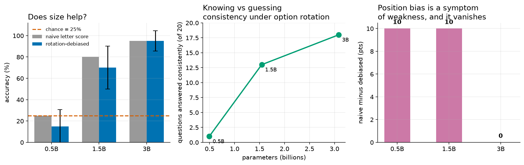— Figure 1:The size ladder, measured. Three models from one family sat one bank of twenty questions under one procedure. **Left:** accuracy, with the dashed line at the 25% chance level. The smallest model’s debiased score falls below that line. **Middle:** on how many of the twenty questions shuffling the options made no difference to whether the model got them right, which is Section 11.6. **Right:** the gap between the two scoring columns, which closes as the model gets larger. The right-hand panel names a cause, position bias, that this chapter does not explain; Chapter 13 does. Drawn by `lab/fig_ladder.py` from `lab/out/lab4_size_ladder.json`.

The left panel is the table you have already read, drawn. Start with the dashed line, because it is the reference everything else is measured against: that is chance, at 25%. The grey bars are the first scoring procedure and the blue bars are the second. The thin vertical lines sticking out of the blue bars are a way of drawing uncertainty, and they are there to stop you reading the bar tops as exact. What they mean, how they are computed, and why they are so wide on twenty questions is Chapter 12.

What this experiment does not license you to say

It is a controlled experiment and it is honest, and it is still twenty questions.

You may say: on this bank of twenty statistics questions, scored by this procedure, larger models in the Qwen2.5-Instruct family scored higher, and the gain from the first step was larger than the gain from the second.

You may not say: that Qwen2.5-3B-Instruct is 95% accurate. The denominator is missing, and so is the bank, and so is the procedure.

You may not say: that this settles whether the 3B beats the 1.5B. Twenty questions is too few to separate two models reliably. Chapter 12 computes how wide the uncertainty actually is, and Chapter 13 compares those two models properly and finds that a 25 percentage point gap does not clear the bar that the right statistical test sets.

You may not say: that this transfers to any other subject. The bank is introductory statistics. A model that can do statistics multiple-choice may be hopeless at Kern County water law, and nothing here speaks to that.

Python¶

The two scoring columns, the counts, and the models are all in the file that was opened in Section 11.4. Nothing new needs loading.

for one_model_name in model_name_list:
    one_result = ladder_results[one_model_name]
    short_name = one_model_name.replace("Qwen/", "").replace("-Instruct", "")
    # Formula 11.2 applied to each of the two scoring procedures.
    naive_percentage = one_result["naive_accuracy"] * 100
    debiased_percentage = one_result["rotation_accuracy"] * 100
    # Formula 11.1 run backwards: a proportion times the number of questions is a count.
    debiased_count = one_result["rotation_accuracy"] * one_result["n"]
    print(short_name,
          "  naive:", naive_percentage, "percent",
          "  debiased:", debiased_percentage, "percent",
          "  which is", debiased_count, "of", one_result["n"])

Output:

Qwen2.5-0.5B   naive: 25.0 percent   debiased: 15.0 percent   which is 3.0 of 20
Qwen2.5-1.5B   naive: 80.0 percent   debiased: 70.0 percent   which is 14.0 of 20
Qwen2.5-3B   naive: 95.0 percent   debiased: 95.0 percent   which is 19.0 of 20

Every number in that output matches the table above, which matches the file, which was written by the script that ran the models. That chain is the honesty policy of this book made concrete, and you can walk any link of it yourself.

The which is column is Formula 11.1 used in reverse. An accuracy of 0.15 on 20 questions means $0.15 \times 20 = 3$ questions right. Turning a proportion back into a count is the single fastest way to catch a nonsense score: if the count does not come out a whole number, something is wrong with the arithmetic or with the reported figure.

Now the steps between the rungs, which is Formula 11.7 and Formula 11.6 side by side.

# The two steps of the ladder, written out as pairs so nothing is inferred from order.
step_from_list = ["Qwen/Qwen2.5-0.5B-Instruct", "Qwen/Qwen2.5-1.5B-Instruct"]
step_to_list = ["Qwen/Qwen2.5-1.5B-Instruct", "Qwen/Qwen2.5-3B-Instruct"]

for step_position in range(2):
    smaller_result = ladder_results[step_from_list[step_position]]
    larger_result = ladder_results[step_to_list[step_position]]
    smaller_percentage = smaller_result["rotation_accuracy"] * 100
    larger_percentage = larger_result["rotation_accuracy"] * 100
    # Formula 11.7, the gain in percentage points.
    difference_in_points = larger_percentage - smaller_percentage
    # Formula 11.6, what the gain cost in size.
    parameter_ratio = larger_result["params"] / smaller_result["params"]
    print("step", step_position + 1,
          " accuracy went from", smaller_percentage, "to", larger_percentage, "percent",
          " a gain of", difference_in_points, "percentage points",
          " for", round(parameter_ratio, 4), "times the parameters")

Output:

step 1  accuracy went from 15.0 to 70.0 percent  a gain of 55.0 percentage points  for 3.1247 times the parameters
step 2  accuracy went from 70.0 to 95.0 percent  a gain of 25.0 percentage points  for 1.999 times the parameters

There is the diminishing-returns result, printed. Step 1 bought 55.0 points for 3.1247 times the size. Step 2 bought 25.0 points for 1.999 times the size.

Both loops walked the same three models in the same order, and both took their numbers from the same file. Writing the pairs out explicitly in step_from_list and step_to_list, rather than assuming that the next model in the list is the next rung, is slightly more typing and removes a whole class of silent error. When the correctness of a result depends on the order things happen to be in, write the order down.

Try it 11.5: reading the ladder

Use the table in this section. All numbers are real.

(a) Express the largest model’s debiased score as a fraction, a decimal and a percentage.

(b) How many percentage points above chance is the middle model’s debiased score?

(c) A colleague writes: “our experiment shows that tripling model size triples accuracy.” Using the measured numbers, say what is wrong with that sentence.

(d) Suppose a fourth model existed with 6.2 billion parameters, twice the largest. Using only the pattern in this section, what would you predict for its debiased score, and why should you not report that prediction as a result?

11.6 Knowing, and guessing, are different¶

Intuition¶

Imagine two people sitting the same four-option exam.

The first person knows the material. She reads a question, works out that the answer is “4”, finds “4” among the options, and marks it. Now imagine you reprint the exam with the options in a different order, so that “4” has moved from slot B to slot D. She reads it, works out that the answer is “4”, finds “4” in slot D, and marks D. Her answer changed letter. Her answer did not change meaning. She got it right both times.

The second person does not know the material and is working from a feeling about where the right answer usually sits. He marks B. On the reshuffled version he marks B again, because his feeling is about the letter, not about the content. Sometimes B is right and sometimes B is wrong, and which it is has nothing to do with him.

There is the test, and it is beautiful in its simplicity. Move the options around and see whether the model’s verdict moves with them. If a model is reading the options, shuffling them changes which letter it says and does not change whether it is right. If a model is doing something else, shuffling them changes whether it is right, and that change is visible in the data.

This is what the lab did. Every question was put to every model four times under rotation, once with the options in their original order and once for each of the three other rotations. A rotation here means sliding all four options along by one position, with the one that falls off the end coming back around to the front. The correct answer moves with its option, so the lab always knows which slot holds the right answer on each pass.

Those four rotation passes are not the whole bill. The naive column of Section 11.5 was scored on a pass of its own, in the original order, before the rotations began. So each question costs five runs of the model and not four, and that is the number Formula 11.8 works with below.

Then, for each question, the lab looked at the four verdicts. If the model found the correct option on all four passes, or failed to find it on all four passes, the question is counted as consistent: shuffling made no difference. If the model found it on some passes and not others, the question is counted as inconsistent, and that can only happen if moving the options changed the model’s mind.

Here is why this measurement earns its place in a chapter about tests. Accuracy alone cannot tell knowing from guessing. Consistency can. And it does it without a single extra question.

The mathematics¶

Here is the consistency column of the ladder on its own, because it deserves to be looked at without the accuracy numbers shouting over it. All real, from lab/out/lab4_size_ladder.json.

Model	Consistent questions	As a proportion	As a percentage
`Qwen2.5-0.5B-Instruct`	1 of 20	$1 \div 20 = 0.05$	5.0%
`Qwen2.5-1.5B-Instruct`	13 of 20	$13 \div 20 = 0.65$	65.0%
`Qwen2.5-3B-Instruct`	18 of 20	$18 \div 20 = 0.90$	90.0%

That first row is the most informative number in this chapter.

On nineteen of the twenty questions, the smallest model’s verdict flipped when the options were moved. Not the letter it said, which is expected and fine. Whether it was right. Slide the options along by one slot and a question it had correct becomes a question it has wrong, or the other way about.

A model whose correctness depends on where an option was printed is not answering the question. Whatever its accuracy comes out as, whether that is the 25.0% of the naive column or the 15.0% of the debiased column, the number is not measuring knowledge of statistics, because knowledge of statistics does not move when you move a list.

Now read down the column. One, then thirteen, then eighteen. The largest model’s verdict held still on 18 of 20 questions. It is reading the options. Its 95.0% means something.

This is the honest form of the answer to “does size help?” Size did not only raise the score. It changed what the score was made of. The smallest model’s 15.0% and the largest model’s 95.0% are not two points on one scale, because the first is a number produced by a procedure that was not measuring what it claimed to measure, and the second is not.

Where this goes next

The lab did not stop at counting consistency. It used the four rotations to build a score. For each question it looked at the four verdicts and asked how many of them were correct, and it counted the question as correct only if the model found the right option on at least three of the four rotations. Three out of four is a majority of four, so this is a vote, and one lucky pass cannot carry a question on its own. That is the “debiased” column. Taking that procedure apart, comparing it with two others, and showing what each one actually measures, is Chapter 13.

This chapter asks you to carry one observation forward: the gap between the two scoring columns was 10 points, 10 points and 0 points, and the consistency counts were 1, 13 and 18. Those two patterns are related. Working out how is next week.

Formula 11.8: the cost of a scoring procedure, in forward passes¶

1. In words. Every time you ask the model a question, that is one run of the model. Multiply the number of questions by the number of times you ask each one, and you have the total number of runs the procedure costs.

2. The formula.

F \;=\; n \times r

3. The symbols.

Symbol	How to say it out loud	What it means
$F$	“eff”	the answer: the total number of forward passes, which is the total number of times the model has to be run
$=$	“equals”	both sides are the same number
$n$	“en”	how many questions are on the bank
$\times$	“times”	multiply
$r$	“arr”	how many times each question is put to the model. This is a different $r$ from the size ratio in Formula 11.6. Letters get reused, and that is exactly why you read a symbol table before you use a formula.

4. Out loud. “F equals n times r.” In full English: “the number of model runs is the number of questions multiplied by the number of times you ask each one.”

5. Worked, with real numbers. The lab’s procedure asks each question once in its original order, for the naive column, and then once for each of the four rotations, for the debiased column. That is five times in total, and there are twenty questions.

Step 1. $n = 20$ and $r = 5$ .

Step 2. Multiply.

F = 20 \times 5 = 100

One hundred forward passes per model. The script lab/lab4_size_ladder.py prints exactly that number when it runs, and it measured how long those hundred passes took (real, from lab/out/lab4_size_ladder.json, the field infer_s):

Model	Seconds for 100 forward passes	Seconds per forward pass
`Qwen2.5-0.5B-Instruct`	6.38	$6.38 \div 100 = 0.0638$
`Qwen2.5-1.5B-Instruct`	8.06	$8.06 \div 100 = 0.0806$
`Qwen2.5-3B-Instruct`	20.62	$20.62 \div 100 = 0.2062$

Step 3, the comparison that matters for Chapter 7. Divide the largest model’s time per pass by the smallest model’s:

0.2062 \div 0.0638 = 3.23

to two decimal places. The largest model took about 3.23 times as long per question as the smallest, on this machine, for 6.2464 times the parameters.

Worked again, to show what the formula is for. Suppose you wanted the 1,000-question bank that the research literature recommends, scored the same way. This one is made up for practice, because nobody has run it.

F = 1000 \times 5 = 5000

Five thousand forward passes per model. At the largest model’s measured 0.2062 seconds each, that is $5000 \times 0.2062 = 1031$ seconds. A minute holds 60 seconds, so divide by 60 to get minutes: $1031 \div 60 = 17.2$ minutes to one decimal place, for one model on one bank. Multiply by three models and it is $3 \times 17.2 = 51.6$ minutes, under an hour. The measurement most people say is too expensive to do properly is, on a laptop, an afternoon.

6. Check it. $F$ must be a whole number and it must be at least $n$ , because you have to ask every question at least once. If $r$ comes out below 1 you have divided instead of multiplied. And if a published evaluation does not tell you $r$ , you cannot compare its cost, or its rigour, with anybody else’s.

Python¶

The consistency counts are in the same file as everything else, under the label consistent. The block below reads them and turns each one into a percentage. It carries on from Section 11.4, so ladder_results and model_name_list are already loaded and the file is not opened again. The only new thing in it is which number gets divided.

for one_model_name in model_name_list:
    one_result = ladder_results[one_model_name]
    short_name = one_model_name.replace("Qwen/", "").replace("-Instruct", "")
    # Formula 11.1 applied to a different count: consistent questions instead of correct ones.
    consistency_proportion = one_result["consistent"] / one_result["n"]
    print(short_name,
          "  shuffling changed nothing on", one_result["consistent"], "of", one_result["n"], "questions",
          " =", consistency_proportion * 100, "percent")

Output:

Qwen2.5-0.5B   shuffling changed nothing on 1 of 20 questions  = 5.0 percent
Qwen2.5-1.5B   shuffling changed nothing on 13 of 20 questions  = 65.0 percent
Qwen2.5-3B   shuffling changed nothing on 18 of 20 questions  = 90.0 percent

That loop used Formula 11.1 without any modification at all. A proportion is a count divided by a total, and it does not care what is being counted. Correct answers divided by questions gives accuracy. Consistent questions divided by questions gives a consistency rate. Same formula, same division, different meaning, and the meaning lives in your head rather than in the arithmetic.

This is worth sitting with for a moment, because it is a large part of what mathematics is for. One piece of machinery, learned once, serves every situation with the same shape. You learned $\hat{p} = x / n$ for accuracy in Section 11.1 and you have now used it for something else without learning anything new.

The last block puts the cost of the procedure next to the result it bought.

# How many times each question was put to the model: once in the original order,
# then once for each of the four rotations.
times_each_question_was_asked = 5

for one_model_name in model_name_list:
    one_result = ladder_results[one_model_name]
    short_name = one_model_name.replace("Qwen/", "").replace("-Instruct", "")
    # Formula 11.8.
    forward_passes = one_result["n"] * times_each_question_was_asked
    seconds_per_pass = one_result["infer_s"] / forward_passes
    print(short_name,
          " forward passes:", forward_passes,
          " total seconds:", round(one_result["infer_s"], 2),
          " seconds per pass:", round(seconds_per_pass, 4))

Output:

Qwen2.5-0.5B  forward passes: 100  total seconds: 6.38  seconds per pass: 0.0638
Qwen2.5-1.5B  forward passes: 100  total seconds: 8.06  seconds per pass: 0.0806
Qwen2.5-3B  forward passes: 100  total seconds: 20.62  seconds per pass: 0.2062

Those timings come from one run on one machine, a laptop with an NVIDIA RTX 3500 Ada GPU, and they would come out differently on yours. They are printed here because the shape of the pattern survives: the largest model costs several times more per question than the smallest, and that cost is paid on every question, for as long as the model is in service.

That last clause is the bridge to the part of this course that is not about accuracy at all. A model you train once and run a million times pays its running cost a million times. Chapter 7 measures that cost in joules, and finds that this largest model spends 2.53 times the energy per token of the smallest (real, computed from the per-token figures in lab/out/theme_s_energy.json, which are 1.940526 joules per token for the largest model and 0.767069 for the smallest; $1.940526 \div 0.767069 = 2.53$ to two decimal places). Set that beside what you measured here: 6.2464 times the parameters bought 80.0 percentage points of accuracy on this bank, and it costs 2.53 times the energy for every token it will ever write.

Which of those two facts matters more depends on who is paying, and that question is the reason this is a general education course.

Try it 11.6: knowing or guessing

(a) A model is consistent on 8 of 20 questions. Write that as a proportion and as a percentage.

(b) Model X scores 60.0% accuracy and is consistent on 4 of 20 questions. Model Y scores 55.0% accuracy and is consistent on 17 of 20. Which result would you rather report, and why? These figures are made up for practice.

(c) A 50-question bank is scored with each question asked three times. How many forward passes is that? If each pass takes 0.0638 seconds, how long does the whole thing take?

Worked examples¶

The arithmetic inside each formula above was worked one formula at a time. These three examples put several formulas together, the way a real evaluation does. Every step is written down.

Worked example 11.1: scoring a small bank from scratch¶

The situation. These numbers are made up for practice. You give a model a bank of 5 four-option questions. It answers questions 1, 3 and 4 correctly, and gets 2 and 5 wrong. Report the result properly.

Step 1. Count what happened.

Correct: questions 1, 3, 4. That is 3 questions.

x = 3

Asked: questions 1 through 5. That is 5 questions.

n = 5

Step 2. Accuracy, by Formula 11.1.

\hat{p} = \frac{x}{n} = 3 \div 5 = 0.6

Step 3. As a percentage, by Formula 11.2.

P = 0.6 \times 100 = 60.0\%

Step 4. Chance level, by Formula 11.3. Each question has 4 options.

c = 1 \div 4 = 0.25 \quad\text{which is } 25.0\%

Step 5. What a guesser would have got, by Formula 11.4.

E = n \times c = 5 \times 0.25 = 1.25 \text{ questions}

A guesser gets one and a quarter questions right on average. No single run can produce a quarter of a question; the 1.25 is a long-run average across many runs, which is what the word “expected” means in the symbol table of Formula 11.4.

Step 6. How far above chance, by Formula 11.7, with chance as the first value.

d = (0.6 - 0.25) \times 100 = 0.35 \times 100 = 35.0

35.0 percentage points above chance.

Step 7. Write the result the way it should be written.

The model scored 3 of 5, which is 60.0%, on a bank of five four-option questions where chance is 25.0%. That is 35.0 percentage points above chance. Five questions is far too few to conclude anything.

The check. $\hat{p}$ is between 0 and 1. The percentage is between 0 and 100. $E$ is between 0 and $n$ . Turning the accuracy back into a count gives $0.6 \times 5 = 3$ , which is the count we started with. Every arrow points the right way.

Worked example 11.2: the score that was exactly chance¶

The situation. All numbers here are real, from lab/out/we6_eval.json. Qwen2.5-0.5B-Instruct was put through this course’s twenty-question bank under the naive letter-ranking procedure of Section 11.3. The file records "correct": 5 and "n": 20.

Step 1. Accuracy, by Formula 11.1.

\hat{p} = 5 \div 20 = 0.25

Step 2. As a percentage, by Formula 11.2.

P = 0.25 \times 100 = 25.0\%

Step 3. Chance level, by Formula 11.3, with $k = 4$ options.

c = 1 \div 4 = 0.25 \quad\text{which is } 25.0\%

Step 4. Distance above chance, by Formula 11.7.

d = (0.25 - 0.25) \times 100 = 0 \times 100 = 0.0

Zero. Not nearly zero. Zero.

Step 5. What a guesser would have got, by Formula 11.4.

E = 20 \times 0.25 = 5 \text{ questions}

The model got 5. A guesser gets 5.

Step 6. Say what this does and does not mean.

It does not mean the model was guessing. It means this measurement cannot tell the difference between this model and a guesser. Those are different statements and the second one is the defensible one.

It also does not mean the model knows no statistics. It means the naive procedure found no evidence that it does. Change the procedure and the number changes: 35.0% under one repair and 15.0% under another (real, from lab/out/we6b_eval_debiased.json). Three honest procedures on one model and one bank, and none of the three agrees with the others.

The check. A model landing exactly on chance is the loudest alarm in evaluation. When you see it, the first thing to inspect is not the model. It is your scoring code. That instinct, followed through, is Chapter 13.

Worked example 11.3: the whole ladder, from counts to a conclusion¶

The situation. All numbers real, from lab/out/lab4_size_ladder.json. Three models, one bank of $n = 20$ , one procedure. Correct counts under the debiased procedure: 3, 14 and 19.

Step 1. Three accuracies, by Formula 11.1. The small labels written low and to the right of each $\hat{p}$ are subscripts, and here they hold model names instead of numbers. They do the same job the $_1$ and $_2$ did in Formula 11.7: they say which model each accuracy belongs to, and they are not multiplication. See Toolkit 2.

\hat{p}_{0.5B} = 3 \div 20 = 0.15

\hat{p}_{1.5B} = 14 \div 20 = 0.70

\hat{p}_{3B} = 19 \div 20 = 0.95

Step 2. As percentages, by Formula 11.2. Multiply each by 100: 15.0%, 70.0% and 95.0%.

Step 3. The two steps of the ladder, by Formula 11.7.

First step: $(0.70 - 0.15) \times 100 = 0.55 \times 100 = 55.0$ percentage points.

Second step: $(0.95 - 0.70) \times 100 = 0.25 \times 100 = 25.0$ percentage points.

Step 4. What each step cost, by Formula 11.6.

First step: $1{,}543{,}714{,}304 \div 494{,}032{,}768 = 3.1247$ .

Second step: $3{,}085{,}938{,}688 \div 1{,}543{,}714{,}304 = 1.9990$ .

Step 5. Accuracy bought per multiple of size. Divide each gain by its ratio.

First step: $55.0 \div 3.1247 = 17.6$ percentage points per multiple.

Second step: $25.0 \div 1.9990 = 12.5$ percentage points per multiple.

Step 6. The whole ladder in one ratio. From smallest to largest:

3{,}085{,}938{,}688 \div 494{,}032{,}768 = 6.2464 \text{ times the parameters}

(0.95 - 0.15) \times 100 = 80.0 \text{ percentage points of accuracy}

Step 7. The conclusion, stated so that it can be checked.

On twenty introductory statistics questions, scored by rotation-debiased letter ranking, three models of the Qwen2.5-Instruct family scored 15.0%, 70.0% and 95.0%. Chance on this bank is 25.0%. Going from the smallest to the largest is 6.2464 times the parameters for a gain of 80.0 percentage points, and the return per multiple of size fell from 17.6 points on the first step to 12.5 on the second. Twenty questions cannot separate the top two models; see Chapter 12.

The check. Multiply the two step ratios: $3.1247 \times 1.9990 = 6.2463$ , against the direct 6.2464. They agree to three decimal places, and the difference is rounding dust. Add the two step gains: $55.0 + 25.0 = 80.0$ , which matches the whole-ladder gain exactly. Percentage points add. Ratios multiply. Getting those two operations the right way round is most of what goes wrong in tables like this one.

Common mistakes¶

These are the errors that actually happen, in rough order of how often.

Reporting a percentage with no denominator. “95% accurate” is half a claim. Ninety-five percent of twenty is 19 questions and could easily have been 17. Always attach $n$ .
Forgetting that chance is not zero. A 30% score on a four-option test sounds like a failing grade and is barely above a pigeon. A 30% score on a ten-option test is three times chance. Work out the floor before you judge the score.
Confusing percent with percentage points. The middle model beat the smallest by 55.0 percentage points, which is Formula 11.7. It did not beat it by 55%. In relative terms it scored 366.7% more, which is Formula 11.2a. Three numbers, one situation, and only one of them belongs in each sentence. See Toolkit 11a.
Multiplying by 100 in the wrong place. Formula 11.4 takes the chance level as a proportion. Feeding it 25 instead of 0.25 gives $20 \times 25 = 500$ questions right out of 20. Percentages become proportions before they go into a formula, every time.
Getting negative numbers backwards. -6.163 is larger than -8.891. A procedure that picks the most negative log-probability as the winner will confidently report the option the model liked least, and the output will look perfectly plausible.
Comparing scores across different procedures. The same model scored 25.0%, 35.0% and 15.0% on the same twenty questions under three defensible procedures (real, from lab/out/we6b_eval_debiased.json). A score belongs to a procedure. Two numbers produced by different procedures are not comparable, however similar the two tables look.
Comparing scores across different banks. A score belongs to its questions as well. The twenty questions here are introductory statistics. Nothing in this chapter says anything about any other subject.
Treating a measured accuracy as a fixed property of the model. It is a sample proportion, measured on the questions you happened to ask. Ask twenty different questions and you get a different number. This is why $\hat{p}$ wears a hat, and it is the whole of Chapter 12.
Confounding the comparison. If two models differ in size and were also given different prompts, the comparison measures nothing. Write down what you held still before you run anything, not after.
Believing a table you have not checked. Every table you will ever read was printed by somebody’s loop. Do one row by hand. It takes twenty seconds and it is the cheapest quality control in science.

What to remember¶

Accuracy is a proportion: the number of questions the model got right divided by the number you asked, which is a decimal between 0 and 1 and a percentage when you multiply it by 100. A score means nothing until four things are attached to it: how many questions, which questions, which scoring procedure, and what chance level that test has. On our four-option bank, chance is 25.0%, and one of our models scored exactly that. A controlled experiment holds everything still except the one variable you are studying, which is why the three models in this chapter came from one family and sat one bank under one procedure. Size helped, by 80.0 percentage points from the smallest model to the largest, and the return per multiple of size fell as the models grew.

Practice problems¶

Twenty-eight problems in three tiers. Warm-up asks whether you can do the arithmetic. Practice asks whether you can apply it. Stretch asks whether you can reason with it.

Numbers marked real come from a file in lab/out/ and you can check them there. Numbers marked made up for practice were invented for the problem and describe no real model.

Solutions to the odd-numbered problems are collected in Answers, Chapter 11. That appendix fills in behind the chapters, so if a solution is not there yet, the problem set is newer than the appendix.

Warm-up¶

A model answers 7 of 20 questions correctly. Write its accuracy as a fraction, as a decimal, and as a percentage. Made up for practice.
Convert each of these. (a) The proportion 0.45 into a percentage. (b) The percentage 82% into a proportion. (c) The proportion 0.07 into a percentage. (d) The percentage 5% into a proportion.
Work out the chance level, as a proportion and as a percentage, for a multiple-choice test with (a) 4 options, (b) 2 options, (c) 5 options, (d) 8 options.
A four-option test has 40 questions. How many does a guesser get right on average? Use Formula 11.4 and show both numbers you multiplied. Made up for practice.
One model scores 12 of 20 and another scores 15 of 20. Compute both accuracies as percentages and then the difference between them in percentage points. Made up for practice.
Qwen2.5-3B-Instruct scored 0.95 on a bank of 20 questions (real). Turn that proportion back into a count of correct answers, and show the multiplication.
Which of these is the largest number: -3.9, -2.4, -7.1, -2.9? Now say what the argmax of the list $[-3.9,\ -2.4,\ -7.1,\ -2.9]$ is, being careful to give a position and not a value.
A model gives an option the log-probability -2.3. Turn that into a probability using the exp key, then write it as a percentage to two decimal places. Made up for practice.
Using the parameter counts 494,032,768 and 3,085,938,688 (real), compute how many times bigger the second model is than the first, to four decimal places.
Qwen2.5-1.5B-Instruct has 1,543,714,304 parameters (real). At FP16 each parameter takes 2 bytes. Compute the size in bytes, then in gigabytes, counting a gigabyte as 1,000,000,000 bytes.

Practice¶

Under the naive procedure Qwen2.5-0.5B-Instruct scored 25.0% on the 20-question bank (real). How many questions is that? Compare it with the number a guesser gets, and say in one sentence what the comparison tells you and what it does not.
Using the debiased accuracies 15.0%, 70.0% and 95.0% (real), compute how many percentage points above or below chance each model scored. Name the model that is below chance.
The consistency counts are 1, 13 and 18 out of 20 (real). Turn each into a proportion and a percentage. Then say, for the smallest model, how many questions had their verdict changed by shuffling the options.
Using Formula 11.8, compute the number of forward passes needed for (a) a 20-question bank with each question asked 4 times, and (b) a 1,000-question bank with each question asked once. Which costs more, and by how many times? Made up for practice; neither run was done.
A vendor writes: “Our assistant is 92% accurate.” Write down the four things you would need to know before this sentence means anything, and for each one, say what a bad answer would look like.
A model returns these log-probabilities for a four-option question: A $= -5.20$ , B $= -4.10$ , C $= -6.80$ , D $= -4.60$ . Made up for practice. (a) Which option does Formula 11.5 extract? (b) How many times more likely did the model think the winner was than the runner-up? Use the subtract-then-exponentiate shortcut. (c) The right answer is D. Was the model right?
A model scores 18 of 40 on a five-option test. Made up for practice. Compute its accuracy as a percentage, the chance level, and how many percentage points above chance it landed.
The measured time per forward pass was 0.0806 seconds for the 1.5B model and 0.2062 seconds for the 3B model (real, computed from lab/out/lab4_size_ladder.json). How many times slower per question is the larger model? Compare that ratio with the parameter ratio 1.9990 and say what the comparison suggests.
The debiased scores went from 70.0% to 95.0% (real). Compute (a) the gain in percentage points, using Formula 11.7, and (b) the gain as a relative percentage, using Formula 11.2a. Then write one sentence using each number correctly.
You want to compare two language models fairly. Write a list of at least six things you would hold constant, and for each one, name a way the comparison could go wrong if you did not.

Stretch¶

A model scores below the chance level on a multiple-choice bank. Give two different explanations that would produce that result, and for each one describe a measurement that would tell you whether it is the right explanation.
Across the ladder, the two step gains were 55.0 and 25.0 percentage points, and the two size ratios were 3.1247 and 1.9990 (real). Show that the gains add to the whole-ladder gain and that the ratios multiply to the whole-ladder ratio. Then explain, in plain English, why one operation is addition and the other is multiplication.
The gap between the naive and debiased columns was 10 points for the smallest model, 10 points for the middle one, and 0 points for the largest (real). The consistency counts were 1, 13 and 18 out of 20 (real). State a hypothesis linking the two patterns, and name the additional measurement you would want before believing it. You are not expected to be right; you are expected to be checkable.
A computer lab at CSUB has machines with 4 GB of graphics memory and no cloud budget. Using the FP16 sizes 0.988 GB, 3.087 GB and 6.172 GB (real) and the debiased accuracies 15.0%, 70.0% and 95.0% (real), argue for one model to install. Your answer must name what your choice gives up as well as what it buys.
The largest model has 6.2464 times the parameters of the smallest, scores 80.0 percentage points higher on this bank, and spends 2.53 times the energy per token (real, computed from lab/out/theme_s_energy.json). Someone asks whether it is “worth it”. Explain why that question cannot be answered from these three numbers alone, and list what else you would need to know.
A colleague proposes reporting, for each model, whichever of the two scoring columns is higher. Write down the ladder that this would produce, then give two separate reasons why the practice is not allowed. One reason should be about what a score means; the other should be about what happens when everyone does it.
Design an experiment to test the claim “consistency under option rotation keeps rising as models get bigger.” Say which models you would use and why, how many questions and why that number, what you would hold constant, and what result would show the claim to be false. A claim that no possible result could falsify is not a scientific claim, which is the subject of Chapter 14.
Formula 11.7a gave 17.6 percentage points per multiple of size on the first step and 12.5 on the second (real). (a) Recompute both, showing the division. (b) A colleague uses the 12.5 to predict that a model with 1.9990 times the parameters of the 3B would score $95.0 + 12.5 = 107.5\%$ . Say what is wrong with that, using a number. (c) Now say what is wrong with it a second way, using the margins of error from the warning box in Section 11.5. Two separate objections, and a good answer gives both.

Looking ahead¶

You now have a score. Chapter 12 asks whether it is real, and the answer involves putting an interval around every accuracy in this chapter. One of those intervals runs from 6.0% to 44.0% (real, from lab/out/we6_eval.json), which is wide enough to hold the chance level and a score far above it at the same time.

Then Chapter 13 picks up the two columns you have been carrying since Section 11.5 and takes the procedure apart. The same model, the same twenty questions, three defensible scoring procedures, three different answers. That chapter is the reason this course is taught by a mathematics department.