3. What is a parameter? - Inside the Machine: The Mathematics of Small Language Models

You have heard a model described by a number. “A 7 billion parameter model.” “A 0.5B model.” The number is printed on the download page the way a weight is printed on a bag of cement.

This chapter answers the question that number is hiding: a count of what, exactly?

What you need before this chapter¶

This is an honest list. Nothing on it is long, and every item links to the exact place that teaches it from nothing.

From the Math Toolkit:

You will meet	Toolkit section	Why this chapter needs it
a letter standing for a number	Section 1	the formulas below use $N$ for a count of numbers
subscripts, like $N_{\text{total}}$	Section 2	one letter, several jobs, told apart by a label
multiplication written four ways	Section 3	counting a rectangle of numbers is a multiplication
the fraction bar as division	Section 4	a share is one count divided by another
exponents, like 10⁹ and $(\ )^2$	Section 5	a small raised number says how many times to multiply something by itself
square roots	Section 9	the standard deviation ends in one
sigma notation, “add these up”	Section 10	the mean and the standard deviation are both built on it
percentages and decimals	Section 11	0.2756 and 27.56% are the same number in different clothes
reading a graph	Section 13	this chapter has a bar chart with a point to make
rounding, decimal places and significant figures	Section 16	four rounded shares will fail to add up, and that is fine
scientific notation	Section 17	494,032,768 is tiring to read and $4.94 \times 10^{8}$ is not

From Chapter 2: one idea. A token is a piece of text that the model treats as a single unit. The model does not read letters or words. It reads a list of token numbers. The set of all tokens it knows is called its vocabulary, and for the model in this chapter the vocabulary holds 151,936 tokens. That is the whole of Chapter 2 you need here.

From programming: nothing. Every line of Python in this chapter is printed in full and explained line by line. If you have never typed a line of code, start at the Python Reference and come back.

The setup cell¶

Run this once, at the top of your session, before anything else on this page. It is one cell. Every import the chapter uses is in it, one per line, each with a comment saying what it is for.

# Cell 1. The setup cell. Run this once, at the top, and then never again today.

import os                                       # lets Python read and change settings on your computer
os.environ["HF_HOME"] = r"C:\math3219\models"   # the folder your models live in; this line MUST come
                                                # before the transformers import, or it is ignored

import torch                                    # the arithmetic library that language models are built on
import numpy                                    # fast arithmetic over very long lists of numbers
from transformers import AutoModelForCausalLM   # loads a model that predicts the next token

Three notes on that cell, because two of the lines are easy to get wrong.

os.environ["HF_HOME"] = ... tells the model library where to keep downloaded models. The letter r in front of the quotation marks means “read the backslashes as backslashes.” Windows paths are full of backslashes and Python normally treats a backslash as an instruction. The r switches that off. On a Mac or on Linux your path has forward slashes and the r does no harm.

The order matters. transformers reads HF_HOME at the moment it is imported. Setting it afterwards has no effect, and the model quietly downloads into a folder you did not choose.

import numpy brings in a library for arithmetic over long lists. You will use it once, in Section 3.4, to ask a question about 802,816 numbers at the same time.

The story this chapter starts from¶

Drive out of Bakersfield in any direction and you pass things that are counted. Kern County counts acres of almonds and pistachios. It counts barrels. It counts acre-feet of water in the Kern River. The number on the outside of a thing is how the county talks about the thing.

Nobody here is fooled by a big number on its own. “Four hundred thousand acre-feet” means nothing until you ask of what, measured how, in what year. A number without a unit is not information. It is a mood.

Language models are sold with a number on the outside and no unit at all. The model this course uses is called Qwen2.5-0.5B-Instruct, and the 0.5B in the middle of the name means “about half a billion parameters.” Half a billion of what?

Here is what happens when you find out. You sit in the Walter Stiern Library with a laptop on campus wifi, you type four lines of Python, and a progress bar fills. When it stops, there are 999,587,685 bytes on your hard drive that were not there before. A gigabyte is one thousand million bytes, so to say that in gigabytes you divide by one thousand million. The sign $\div$ says “divided by”, and it is the same instruction as a fraction bar (Math Toolkit Section 4): $999{,}587{,}685 \div 1{,}000{,}000{,}000 = 0.999587685$ , which rounds to 1.00 gigabytes. Section 3.5 takes that conversion apart properly. The byte count was measured on the course machine and recorded in lab/out/appendix_python_reference_checks.json.

That file is not locked. It is not a program. It is not, whatever anyone has told you, a brain. It is a list of numbers, and you are allowed to open it and read them.

There are 494,032,768 of those numbers. Each one is a parameter. By the end of this chapter you will know what each one is, where each one sits, what a typical one looks like, and why the whole pile takes up almost exactly one gigabyte.

And you will meet one genuine surprise. Attention is the part of a language model that gets written about. It has papers named after it. In this model, all of attention together is 8.92 per cent of the parameters. Meanwhile 27.56 per cent of the model, over a quarter of it, is a lookup table for words. The famous part is under a tenth of the machine.

Where the numbers in this chapter come from

Almost every measured number on this page was produced by lab/ch03_parameter_anatomy.py, running Qwen2.5-0.5B-Instruct at 32-bit precision on the course machine, and written to lab/out/ch03_parameter_anatomy.json. You can open that file. The same figures appear in _research/00-lab-verified-findings.md, section 4.

Six numbers on this page come from four other measurements, and each one names its own file where it appears: the size of the download, in lab/out/appendix_python_reference_checks.json; the parameter counts of the two larger models, in lab/out/theme_s_energy.json; the quantization errors quoted ahead to Chapter 7, in lab/out/we3b_quant.json and in section 5 of _research/00-lab-verified-findings.md; and the three Chapter 13 scores, in lab/out/we6_eval.json and lab/out/we6b_eval_debiased.json.

Some worked examples on this page use small invented numbers, because 1, 3, 5, 7 and 9 are easier to check on a phone than 802,816 real weights. Those examples say made up for practice in their first line. Everything else is what the model actually holds.

The book’s rule, which this chapter follows without exception: we never publish a number we did not compute.

Learning objectives¶

By the end of this chapter you will be able to:

(Explain) Say what a parameter is in one sentence, and say what a parameter is not, without using the word “parameter.”
(Apply) Count the numbers in a weight matrix from its shape, and compute what share of a whole model any named part of it holds.
(Apply) Describe a set of hundreds of thousands of weights with a mean, a standard deviation and a median, and say what each of those three tells you that the other two do not.
(Apply) Convert a parameter count into a file size in bytes and gigabytes at four storage formats, and write both the count and a single weight in scientific notation.
(Analyse) Read the parameter inventory of a real model and explain why the popular story about which part matters is not the story the inventory tells.

This lesson at a glance¶

A parameter is one number, set during training, stored in a file, and unchangeable by you.
Those numbers are arranged into rectangles called weight matrices, and you count the numbers in a rectangle by multiplying its rows by its columns.
Sorting all 494,032,768 of them by the part they belong to gives an inventory that contradicts the popular story: 27.56% vocabulary table, 63.51% MLP blocks, 8.92% attention.
A parameter count becomes a physical file size the moment you choose how many bytes to spend on each number, which is why this model arrives as a 1 GB download.

The vocabulary of this chapter¶

Every term below is used later on this page. They are collected here first so that no sentence later on asks you to know something you have not been told.

Term	What it means, in one line
parameter	one number inside a model, set by training and fixed afterwards
weight	another word for a parameter, used when you are looking at the number itself
training	the one-time process, run by somebody else, that chose all the numbers
matrix	a rectangle of numbers, arranged in rows and columns
weight matrix	a matrix whose entries are parameters
row	one horizontal line of numbers in a matrix
column	one vertical line of numbers in a matrix
shape	the pair of counts (rows, columns) that says how big a matrix is
tensor	the word the code uses for a block of numbers, of any shape
token	a piece of text the model treats as one unit, from Chapter 2
vocabulary	the full set of tokens a model knows. 151,936 of them here
vocabulary table	the matrix with one row per token, called `embed_tokens` in the code
hidden size	how many numbers the model uses to carry one token through itself. 896 here
layer	one repeated stage of the model. This model has 24 stacked layers
attention	the part of a layer that looks back at earlier tokens and decides how much weight to give each one
projection	one weight matrix inside attention. There are four: `q_proj`, `k_proj`, `v_proj`, `o_proj`
bias	a small extra row of parameters that some matrices carry, one number per output. Counted with the matrix
MLP block	the wide part of a layer that every token passes through on its own. Three matrices: `gate_proj`, `up_proj`, `down_proj`
layer norm	a small set of parameters that keeps the numbers flowing through a layer at a steady size
share	one count divided by a total, usually written as a percentage
mean	the average of a list of numbers: the total, divided by how many there are
standard deviation	a typical distance from the mean, in the same units as the numbers
absolute value	a number with its minus sign removed, written $\lvert w \rvert$
median absolute value	the middle value once every weight has had its sign removed
bit	one yes-or-no answer, a 0 or a 1, the smallest piece of information there is
byte	eight bits
storage format	the agreement about how many bytes each number gets. FP32, FP16 and INT8 here
FP32	four bytes per number. Also called full precision or single precision
FP16	two bytes per number. Also called half precision
INT8	one byte per number, holding a whole number rather than a fraction
scientific notation	writing a number as something between 1 and 10 times a power of ten
setting	something you choose when you run the model, such as temperature. Not a parameter

3.1 A parameter is one number¶

Intuition¶

Think about a light switch with a dimmer. The dimmer has one position. That position is a single number: say 0.62, on a scale from 0 to 1. The dimmer does not contain a plan or an idea. It holds a number, and the number affects what the lamp does.

Now imagine a room with 494,032,768 dimmers on the wall. Each one holds its own number. None of them knows anything. But the numbers were not set at random. Somebody ran an enormous process that nudged each dimmer, over and over, until the whole wall of them produced useful text. Then they stopped, wrote all 494,032,768 positions into a file, and published the file.

That is a language model. The wall of dimmers is the model, each dimmer is a parameter, and the file of positions is what you downloaded.

Two things follow, and both matter more than they look.

First: you cannot change a parameter by typing. People say they “adjusted the parameters” when they changed the temperature setting or the length of the reply. Those are not parameters. Those are settings you choose at run time. A parameter was set by training, which happened months ago, on somebody else’s machines, and finished. When you run the model tonight, all 494,032,768 numbers are exactly what they were when the file was published, and exactly what they will be tomorrow.

Second: a parameter has no meaning on its own. Open the file, pull any one number out of it, and look at that number. Section 3.3 does exactly this, and the second number it finds is -0.00521851. That is not a fact about France. It is not a rule of grammar. Nothing in it is about anything. The behaviour you see comes out of hundreds of millions of these interacting, the way a photograph comes out of millions of grains of silver, none of which is a picture of anybody.

This is the honest version of “how does a language model work,” and it is available to you today, in Chapter 3, because the file is on your disk and you can print the numbers.

A parameter is not a setting you choose

Three different things get called parameters in ordinary conversation. This book keeps them apart, on purpose, and always names which one is in play.

A parameter, in this chapter’s sense: a learned number inside the model file.
A setting, chosen by you when you run the model: temperature, how many tokens to generate, the random seed. Chapter 5 is about one of these. This book calls them settings, never parameters.
A population parameter, in statistics: a fixed unknown quantity you are trying to estimate, such as a model’s true accuracy over every question you might have asked. Chapters 11 to 14 use this sense and announce it each time.

If someone tells you they “tuned the parameters” of a model they downloaded, they almost certainly changed a setting. Changing a real parameter means retraining.

The mathematics¶

Parameters are not stored as one long list. They are stored in rectangles. A rectangle of numbers, arranged in rows and columns, is called a matrix, and the first thing you ever need to do with one is count how many numbers are inside it.

Formula 3.1. How many numbers are in a matrix

1. In words. A matrix is a grid. To find out how many numbers are in a grid, multiply the number of rows by the number of columns. It is the same arithmetic as working out how many seats are in a lecture hall from the number of rows of seats and the number of seats per row.

2. The formula.

N_{\text{matrix}} = (\text{rows}) \times (\text{columns})

3. The symbols.

Symbol	How to say it out loud	What it means
$N$	“en”	a count of numbers. $N$ is the letter this book always uses for a count of parameters.
the subscript in $N_{\text{matrix}}$	“sub matrix”	a label glued to the letter, saying which count this is. It is not multiplication and it is not a power.
$=$	“equals”	the thing on the left is the same number as the thing on the right
$\text{rows}$	“rows”	how many horizontal lines of numbers the rectangle has
$\times$	“times”	multiply the thing on the left by the thing on the right
$\text{columns}$	“columns”	how many vertical lines of numbers the rectangle has
the round brackets $(\ )$	“bracket”	they hold a quantity together so you can see it counts as one thing
$-$	“minus”	take the thing on the right away from the thing on the left. The formula itself does not use it, but the worked example below does, twice.

4. Out loud. “The number of parameters in a matrix equals its number of rows, times its number of columns.”

5. Worked, with real numbers. The first attention query matrix in this model is called layers[0].self_attn.q_proj.weight, and its shape is (896, 896).

Step 1, write the two numbers down. rows $= 896$ , columns $= 896$

Step 2, multiply. On a calculator that is one keystroke. On paper, split 896 into $900 - 4$ , because multiplying by 900 is easy:

$896 \times 900 = 806{,}400$

$896 \times 4 = 3{,}584$

Step 3, subtract the second from the first, because you used 900 where you wanted 896.

$806{,}400 - 3{,}584 = 802{,}816$

N_{\text{matrix}} = 802{,}816

One matrix. 802,816 numbers. And this model contains 24 of these, plus everything else.

6. Check it. Two tests. The answer must be a whole number, because you cannot have half a number stored in a file. And the answer must be at least as large as the larger of the two sides: 802,816 is far bigger than 896, so the multiplication went the right way. If your answer came out as 1,792, you added the two sides instead of multiplying them.

Worked example 3.1. The vocabulary table

The biggest single matrix in this model is the vocabulary table, the grid that holds one row for each token the model knows. Its shape is (151936, 896): one row per token in the vocabulary, and 896 columns, because 896 is this model’s hidden size, the number of numbers it uses to carry one token through itself.

Step 1, write the two numbers down. rows $= 151{,}936$ , columns $= 896$

Step 2, split the awkward side. Use $896 = 900 - 4$ again.

$151{,}936 \times 900 = 136{,}742{,}400$

$151{,}936 \times 4 = 607{,}744$

Step 3, subtract.

$136{,}742{,}400 - 607{,}744 = 136{,}134{,}656$

N_{\text{vocabulary table}} = 136{,}134{,}656

136,134,656 numbers in one table. Hold on to that figure. Section 3.2 divides it by the size of the whole model and gets the most surprising number in this chapter.

Check it. The answer must be larger than 151,936, and it is. A rough size check also works: 150,000 times 900 is about 135 million, and 136,134,656 is about 136 million. Close enough to believe the long multiplication.

Python¶

Here is the whole of Section 3.1 in code. It loads the model and counts every number in it.

# Cell 2. Load the model, then count every number inside it.

model_name = "Qwen/Qwen2.5-0.5B-Instruct"                  # who published it, and which model
language_model = AutoModelForCausalLM.from_pretrained(     # fetch it, or read it from your disk
    model_name,
    dtype=torch.float32)                                   # keep every number at four bytes, so
                                                           # your digits match the book's digits
language_model.eval()                                      # switch it out of training mode

parameter_count = 0                                        # start the tally at nothing
for one_parameter_block in language_model.parameters():    # walk through the model's blocks
    parameter_count = parameter_count + one_parameter_block.numel()
                                                           # .numel() is "number of elements",
                                                           # that is, how many numbers this block holds

print("model name      :", model_name)
print("parameters      :", parameter_count)
print("vocabulary size :", language_model.config.vocab_size)
print("hidden size     :", language_model.config.hidden_size)
print("layers          :", language_model.config.num_hidden_layers)

Output:

model name      : Qwen/Qwen2.5-0.5B-Instruct
parameters      : 494032768
vocabulary size : 151936
hidden size     : 896
layers          : 24

Now line by line, because most of what you need to know about this chapter is in those eleven lines.

model_name is a piece of text, called a string in Python, holding the model’s address. The part before the slash, Qwen, is the organisation that published it. The part after the slash names the model. The 0.5B is the claim this chapter is testing.

AutoModelForCausalLM.from_pretrained(...) is the line that does the work. Pretrained means somebody else already ran the training, at very large expense, and you are collecting the finished file. The first time you run this, it downloads. Every time after that, it reads from the folder you named in Cell 1, in a second or two.

dtype=torch.float32 says to hold every number at four bytes of precision. This is not what the file on disk uses, and Section 3.5 comes back to that difference. Use it here so that the digits you see match the digits printed in this book.

language_model.eval() switches the model out of training mode. Some parts of a model behave differently while it is being learned. You are not training it, so you say so.

Then the count. parameter_count = 0 starts a tally at nothing. The for loop walks through the model one block of numbers at a time. Each block is a tensor, which is the word the code uses for a block of numbers of any shape. .numel() is short for “number of elements”, and it asks a block how many numbers it holds. The line inside the loop takes the running total, adds this block’s count, and stores the result back in parameter_count.

When the loop ends, parameter_count holds 494,032,768.

That is the answer to “0.5B of what.” It is a count of individual numbers, arranged in rectangles, sitting in a file on your disk. The last three printed lines are the facts the rest of the chapter is built on: the model knows 151,936 tokens, it carries each one as 896 numbers, and it has 24 stacked layers.

3.2 Where 494,032,768 numbers actually live¶

Intuition¶

Take the cover off a machine you have never seen inside and your first question is which part is biggest. Not which part is cleverest. Which part takes up the room.

If you had only read about language models, you would expect the biggest part to be attention. Attention is what the papers are named after. Attention is the thing people gesture at when they explain why these models are good. It is genuinely the mechanism that makes the architecture work, and Chapter 4 onwards will show you what it does.

It is 8.92 per cent of this model.

The biggest single component, by a wide margin once you group the layers together, is the set of MLP blocks, at 63.51 per cent. The second is the vocabulary table, at 27.56 per cent. The vocabulary table is a lookup table. One row per token, 151,936 rows, and the row for token number 8,312 holds the numbers the model uses to stand in for that token. Token 8,312 is akers, the middle piece of Bakersfield from Chapter 2. It is the least mysterious object in the entire machine. It is over a quarter of it.

This is worth sitting with, because it changes what “a bigger model” means. When a company publishes a model with more parameters, the extra numbers are not mostly going into the famous part. They are going into wide, plain layers of arithmetic, and into a table.

It also changes what you should expect of the small model in this course. A model that spends more than a quarter of itself on a vocabulary table and under a tenth on attention is a model that has a lot of storage for individual tokens and not much machinery for relating them to each other. In Chapter 13 you will watch this model score 15 per cent, 25 per cent or 35 per cent on the same twenty questions depending on how you score it, and none of those is good. Twenty questions is a small test, so each of those three scores carries a wide band of uncertainty around it: the 25 per cent score, measured in lab/out/we6_eval.json, comes with a 95 per cent interval running from 6.0 per cent to 44.0 per cent. Chapter 12 builds that interval from nothing and Chapter 13 uses it. Until then, read the three scores as rough, and never read any accuracy in this book without the interval printed beside it. The inventory in this section is one honest place to start looking for why the scores are low.

The mathematics¶

To say “the vocabulary table is 27.56 per cent of this model” you need one piece of arithmetic: dividing a part by a whole.

Formula 3.2. The share of the parameters held by one part

1. In words. Take how many numbers are in one named part of the model. Divide it by how many numbers are in the whole model. That fraction is the part’s share. Multiply by 100 if you want it as a percentage.

2. The formula.

\text{share} = \frac{N_{\text{component}}}{N_{\text{total}}}

3. The symbols.

Symbol	How to say it out loud	What it means
$\text{share}$	“share”	the answer. A number between 0 and 1.
$=$	“equals”	the thing on the left is the same number as the thing on the right
$N_{\text{component}}$	“en sub component”	how many parameters are in one named part, such as all of attention
$N_{\text{total}}$	“en sub total”	how many parameters are in the whole model. Here, 494,032,768.
the fraction bar	“divided by”	divide the number written on top by the number written underneath
$\div$	“divided by”	the same instruction as the fraction bar, written on one line instead of two. $a \div b$ and $\frac{a}{b}$ mean the same thing, and the worked example below uses this form because that is how you type it into a calculator.
the subscripts	“sub component”, “sub total”	labels that say which $N$ each one is. Not multiplication, not a power.

4. Out loud. “The share held by a component equals the number of parameters in that component, divided by the number of parameters in the whole model.”

5. Worked, with real numbers. Work out the share held by all of attention.

Attention is not one matrix. It is four, in every one of the 24 layers, and the measured totals across all 24 layers are these:

projection	parameters across all 24 layers
`self_attn.q_proj`	19,289,088
`self_attn.o_proj`	19,267,584
`self_attn.k_proj`	2,755,584
`self_attn.v_proj`	2,755,584

One thing in that table needs explaining before you use it, because it will not survive a check otherwise. q_proj and o_proj are both 896 by 896 matrices, so Formula 3.1 gives each of them 802,816 numbers, and $802{,}816 \times 24 = 19{,}267{,}584$ across the 24 layers. That is exactly the o_proj figure. The q_proj figure is 21,504 larger. The extra numbers are a bias: a small extra row that some matrices carry, holding one number for each of the 896 outputs. So q_proj holds $802{,}816 + 896 = 803{,}712$ numbers per layer, and $803{,}712 \times 24 = 19{,}289{,}088$ , which is the figure in the table. The difference is $19{,}289{,}088 - 19{,}267{,}584 = 21{,}504$ , and $21{,}504 \div 24 = 896$ , one bias number per output per layer. k_proj and v_proj carry biases too, and Practice problem 16 has you check one of them. o_proj does not.

Step 1, add the four together. Do it two at a time so nothing goes wrong.

$19{,}289{,}088 + 19{,}267{,}584 = 38{,}556{,}672$

$38{,}556{,}672 + 2{,}755{,}584 = 41{,}312{,}256$

$41{,}312{,}256 + 2{,}755{,}584 = 44{,}067{,}840$

So $N_{\text{component}} = 44{,}067{,}840$ .

Step 2, write down the total.

$N_{\text{total}} = 494{,}032{,}768$

Step 3, divide. Type it into a calculator exactly as written.

$44{,}067{,}840 \div 494{,}032{,}768 = 0.0892002$

Step 4, turn the decimal into a percentage by multiplying by 100. Multiplying by 100 moves the decimal point two places to the right.

$0.0892002 \times 100 = 8.92002$

\text{share of attention} = 8.9200\%

6. Check it. A share must land between 0 and 1 before you convert it, and between 0% and 100% after. If you get a number larger than 1, you divided the whole by the part instead of the part by the whole; swap the top and the bottom and try again.

There is a second, better check. Work out the share for every part and add them up. They must come to 100%. Section 3.2’s Python does exactly that, and the honest wrinkle in that check is worth its own warning box below.

Worked example 3.2. One MLP projection

Each of the 24 layers holds three MLP matrices. One of them is called gate_proj, and its shape is (4864, 896), because this model’s MLP blocks widen each token from 896 numbers out to 4,864 before narrowing it again.

Step 1, count one matrix, using Formula 3.1.

$4{,}864 \times 896 = 4{,}358{,}144$

If you want that by hand, split again: $4{,}864 \times 900 = 4{,}377{,}600$ , and $4{,}864 \times 4 = 19{,}456$ , and $4{,}377{,}600 - 19{,}456 = 4{,}358{,}144$ .

Step 2, there are 24 layers, so multiply by 24.

$4{,}358{,}144 \times 24 = 104{,}595{,}456$

Step 3, divide by the model total, using Formula 3.2.

$104{,}595{,}456 \div 494{,}032{,}768 = 0.211718$

Step 4, multiply by 100.

$0.211718 \times 100 = 21.1718$

\text{share of one MLP projection} = 21.1718\%

One of the three MLP matrices is more than twice the size of all of attention. There are three of them.

Check it. $21.1718 \times 3 = 63.5154$ , and the measured total for all three MLP matrices is 63.5153%. Those two do not match in the last digit, and that is a rounding effect, not a mistake. The warning box below says why.

Rounded shares will not add up, and that is not an error

The four attention shares, each rounded to four decimal places, are 3.9044%, 3.9001%, 0.5578% and 0.5578%. Add them:

$3.9044 + 3.9001 + 0.5578 + 0.5578 = 8.9201$

But the share of attention computed from the exact counts is 8.9200%. The two differ by 0.0001 percentage points.

Nothing is wrong. Each of the four numbers was rounded before being added, and four small roundings can lean the same way. Rounding first and adding second is not the same as adding first and rounding second.

The rule to carry out of here: round at the end, never in the middle. When your own numbers fail to add up by a digit in the last place, check whether you rounded early before you go looking for a real mistake. And when they fail to add up by a lot, that is a real mistake.

One note on how this book writes divisions down. A line like $44{,}067{,}840 \div 494{,}032{,}768 = 0.0892002$ has an ordinary equals sign, but the right-hand side has been cut off after seven decimal places; your calculator will keep going, 0.08920023701 and onwards. Every division in this chapter that ends in a decimal is written that way. It means “equal as far as the digits shown”, and where the gap matters, as it does in the four attention shares above, this book says so.

Python¶

Sorting 494,032,768 numbers into the parts they belong to sounds heavy. It is one loop.

# Cell 3. Sort every parameter into the part of the model it belongs to.

parameters_in_part = {}                                      # an empty tally, one slot per part
for parameter_name, parameter_block in language_model.named_parameters():
    if "embed_tokens" in parameter_name:                     # the vocabulary lookup table
        part_name = "embed_tokens"
    elif "mlp.gate_proj" in parameter_name:                  # the three wide MLP matrices
        part_name = "mlp.gate_proj"
    elif "mlp.up_proj" in parameter_name:
        part_name = "mlp.up_proj"
    elif "mlp.down_proj" in parameter_name:
        part_name = "mlp.down_proj"
    elif "self_attn.q_proj" in parameter_name:               # the four attention projections
        part_name = "self_attn.q_proj"
    elif "self_attn.o_proj" in parameter_name:
        part_name = "self_attn.o_proj"
    elif "self_attn.k_proj" in parameter_name:
        part_name = "self_attn.k_proj"
    elif "self_attn.v_proj" in parameter_name:
        part_name = "self_attn.v_proj"
    else:                                                    # anything left over
        part_name = "layer norms"
    if part_name in parameters_in_part:                      # already seen this part before
        parameters_in_part[part_name] = parameters_in_part[part_name] + parameter_block.numel()
    else:                                                    # first time seeing this part
        parameters_in_part[part_name] = parameter_block.numel()

part_names_largest_first = sorted(parameters_in_part, key=parameters_in_part.get, reverse=True)

print("part                 parameters      share")
for part_name in part_names_largest_first:
    share_of_model = 100 * parameters_in_part[part_name] / parameter_count
    print(f"{part_name:<18} {parameters_in_part[part_name]:>12,}  {share_of_model:8.4f}%")

Output:

part                 parameters      share
embed_tokens        136,134,656   27.5558%
mlp.gate_proj       104,595,456   21.1718%
mlp.up_proj         104,595,456   21.1718%
mlp.down_proj       104,595,456   21.1718%
self_attn.q_proj     19,289,088    3.9044%
self_attn.o_proj     19,267,584    3.9001%
self_attn.k_proj      2,755,584    0.5578%
self_attn.v_proj      2,755,584    0.5578%
layer norms              43,904    0.0089%

The pieces of that cell, in order.

parameters_in_part = {} makes an empty dictionary, which is a tally with names instead of positions. You will put a running total under each part’s name.

language_model.named_parameters() is the same walk as Cell 2, except that each step now hands you two things: the block’s name, which is a piece of text like model.layers.7.self_attn.k_proj.weight, and the block of numbers itself.

The long if and elif chain reads each name and decides which bucket it belongs in. elif is short for “else if”, and the chain stops at the first line that is true. The final else catches everything the earlier tests missed, which for this model is the layer norms: small sets of parameters that keep the numbers flowing through each layer at a steady size. There are 43,904 of them, which is 0.0089% of the model.

The two lines at the bottom of the loop do the tallying. If a part already has a running total, add this block to it. If it does not, start it at this block’s count. There are 24 layers, so each attention and MLP bucket gets 24 visits.

sorted(..., reverse=True) puts the parts in order, largest first.

The print inside the last loop uses an f-string, which is a piece of text with slots in it marked by curly brackets. {part_name:<18} means “print the part name, padded out to 18 characters, pushed to the left.” {...:>12,} means “12 characters wide, pushed right, with commas between the thousands.” {share_of_model:8.4f} means “8 characters wide, 4 digits after the decimal point.” Those formats are what makes the output line up into columns.

Nine rows is more detail than the eye wants. Group them.

# Cell 4. Roll those eight parts up into three families, plus the leftovers.

word_table_parameters = parameters_in_part["embed_tokens"]   # one table, one number

mlp_parameters = 0                                           # add the three MLP matrices
mlp_parameters = mlp_parameters + parameters_in_part["mlp.gate_proj"]
mlp_parameters = mlp_parameters + parameters_in_part["mlp.up_proj"]
mlp_parameters = mlp_parameters + parameters_in_part["mlp.down_proj"]

attention_parameters = 0                                     # add the four attention projections
attention_parameters = attention_parameters + parameters_in_part["self_attn.q_proj"]
attention_parameters = attention_parameters + parameters_in_part["self_attn.k_proj"]
attention_parameters = attention_parameters + parameters_in_part["self_attn.v_proj"]
attention_parameters = attention_parameters + parameters_in_part["self_attn.o_proj"]

everything_else_parameters = parameter_count - word_table_parameters - mlp_parameters - attention_parameters

print("family               parameters      share")
print(f"{'word table':<18} {word_table_parameters:>12,}  {100*word_table_parameters/parameter_count:8.4f}%")
print(f"{'MLP blocks':<18} {mlp_parameters:>12,}  {100*mlp_parameters/parameter_count:8.4f}%")
print(f"{'all attention':<18} {attention_parameters:>12,}  {100*attention_parameters/parameter_count:8.4f}%")
print(f"{'everything else':<18} {everything_else_parameters:>12,}  {100*everything_else_parameters/parameter_count:8.4f}%")

Output:

family               parameters      share
word table          136,134,656   27.5558%
MLP blocks          313,786,368   63.5153%
all attention        44,067,840    8.9200%
everything else          43,904    0.0089%

That cell is written out the long way on purpose. Four separate addition lines are easier to read, and easier to check, than one clever line. The book’s style is to repeat rather than to compress, because you can see a repeated line and check it.

The last line works out everything_else_parameters by subtraction rather than by adding things up. That is deliberate, and it is a free error check: if the three families and the leftovers do not add back to 494,032,768, something was miscounted. Add the four printed counts yourself and you get exactly 494,032,768. Add the four printed shares and you get $27.5558 + 63.5153 + 8.9200 + 0.0089 = 100.0000$ .

Read the third line again. All of attention, across all 24 layers, all four projections: 44,067,840 parameters. To ask how many times larger one count is than another, you divide the larger by the smaller. The word table on its own is 136,134,656, so

$136{,}134{,}656 \div 44{,}067{,}840 = 3.0892$

and the word table is 3.0892 times the size of all of attention. The MLP blocks are 313,786,368, so

$313{,}786{,}368 \div 44{,}067{,}840 = 7.1205$

and they are 7.1205 times the size of all of attention.

The picture¶

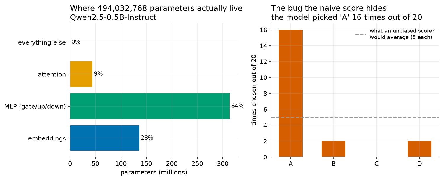
A figure with two panels side by side. The LEFT panel, which is the one this chapter — uses, is a horizontal bar chart titled “Where 494,032,768 parameters actually live, Qwen2.5-0.5B-Instruct”. Its horizontal axis is labelled “parameters (millions)” and runs from 0 to about 300. Four bars run upward from the bottom: embeddings, a blue bar reaching about 136 million and labelled 28 percent; MLP (gate/up/down), a green bar reaching about 314 million and labelled 64 percent, by far the longest; attention, an orange bar reaching about 44 million and labelled 9 percent; and everything else, a bar so short it is invisible, labelled 0 percent. The RIGHT panel belongs to Chapter 13 and is a vertical bar chart of how often the model chose each answer letter, with A chosen 16 times out of 20, B twice, C never and D twice, against a dashed grey line at 5. :width: 100%

Two things to notice in the left panel, and one trap.

The green MLP bar is the longest, and it is longer than the blue embeddings bar and the orange attention bar put together. The orange attention bar is about a third of the blue one.

The trap is the fourth bar. “Everything else” is drawn at 0 per cent and looks like an empty row. It is not empty. It holds 43,904 real parameters, and if you deleted them the model would stop working. A bar chart with a 300-million-wide axis cannot show a 43,904-long bar. A figure shows you the shape; a table gives you the number. This book prints both, and when they disagree about something small, the table is right.

The simulation¶

The bar chart above is fixed. The one below is not. Every bar is one component, and the slider underneath changes the storage format, which is the subject of Section 3.5.

Do one thing with it before you read on. Drag the slider from 0 to 3 and watch the bars. Not one of them moves. The model on disk goes from 1.976 GB down to 0.247 GB, and the shape of the chart is identical. Storing each number in fewer bits does not move a single parameter into a different part of the model. It only shrinks the box each number sits in. That is the whole idea of Chapters 6 and 7, and you can see it here in one drag.

Try it 3.1. Count the leftovers yourself

The layer norms row shows 43,904 parameters. This model has 24 layers, each layer has two layer norms, each layer norm holds one number for each of the 896 numbers the model carries a token in, and then there is one final layer norm at the very end of the model.

Work out 43,904 from those facts, showing each step. Then work out its share of the model as a percentage to four decimal places.

3.3 Opening one real matrix and looking inside¶

Intuition¶

You now know there are 494,032,768 numbers and you know which drawers they are in. You have not yet seen one.

So open a drawer. Take layers[0].self_attn.q_proj.weight, the first attention query matrix in the first layer, 896 rows by 896 columns, 802,816 numbers. Print the first five numbers in the first row and look at them.

They are small. They hover near zero, some positive, some negative, none of them anything like a round number. There is no pattern a person can see in five of them, and there is no pattern a person can see in eight hundred thousand of them either. That is what a trained weight matrix looks like: a haze.

This is the moment a lot of people expect something and do not get it. They expect the numbers to mean something individually. They do not. The meaning is in the whole arrangement, and the arrangement is too big to look at.

So you do what any scientist does with a pile of measurements too large to look at. You summarise it. A summary is a small number of numbers that stand in for a large number of numbers, and the first question any summary answers is where the pile sits.

That is what the mean is for. Add every weight up, divide by how many there are, and you get one number saying where the middle of the pile is. Alongside it, two more facts cost nothing to collect: the single smallest weight in the matrix and the single largest. Those two say how far the pile reaches at each end.

Three numbers, then, in this section: the middle, the far left, and the far right. They turn out to disagree with each other in an interesting way, and that disagreement is what Section 3.4 picks up.

The mathematics¶

One formula in this section: the mean. It is built from sigma notation, which means “add these up”, and it is also worked in full in the Math Toolkit.

Before the formula, one question about it: why bother taking the mean of a weight matrix at all? The mean of 802,816 numbers that individually mean nothing might itself look like it means nothing.

It is worth taking for two reasons, and both are the kind of reason that comes up again in every later chapter.

A summary is a check. You did not train this model and you did not write the file. The mean is one cheap question you can ask of somebody else’s work. If the mean of a trained weight matrix came out at 8, or at 0.4, you would know something had gone wrong before you ran a single word of text through the model. The mean coming out at -0.000017 is a small piece of evidence that the file on your disk is what it claims to be.

A summary is a place to start. Sections 3.4 onwards ask sharper questions: how spread out are these weights, how big is a typical one, are there any strange ones. Every one of those questions is phrased relative to the mean. You need the middle before you can say how far from the middle anything is.

There is a third reason that is worth naming and then setting aside. The mean is also the first formula in this book that runs over a very large number of items. Doing it once by hand on five numbers, as the worked example below does, is what makes the line weight_matrix.mean() in the Python readable rather than magic.

Formula 3.3. The mean of a list of weights

1. In words. Add up every number in the list. Then divide that total by how many numbers were in the list. That is the average.

2. The formula.

\bar{w} = \frac{1}{N}\sum_{i=1}^{N} w_i

3. The symbols.

Symbol	How to say it out loud	What it means
$\bar{w}$	“w-bar”	the mean of the weights. The bar on top means “the average of”.
$=$	“equals”	the two sides are the same number
$\dfrac{1}{N}$	“one over en”	multiplying by one over $N$ is the same as dividing by $N$
$N$	“en”	how many numbers are in the list. Here, 802,816.
$\sum$	“sigma”, or “the sum of”	a capital Greek S. It says: add up whatever comes after me.
$i$	“eye”	a counter. $i = 1$ means the first weight, $i = 2$ the second, and so on.
$i = 1$ underneath the sigma	“i equals one”	where the counter starts
$N$ above the sigma	“en”	where the counter stops
$w_i$	“w sub i”	the $i$ -th weight in the list. The subscript is a position, not a power.
the fraction bar	“divided by”	divide the top by the bottom

4. Out loud. “W-bar equals one over N, times the sum, from i equals one to N, of w sub i.” In plain English: “the mean is the total of all the weights, divided by how many weights there are.”

5. Worked, with real numbers. Use the first five numbers of row 0 of the real matrix, which the code in this section prints:

$w_1 = -0.00193024$ $w_2 = -0.00521851$ $w_3 = +0.01879883$ $w_4 = +0.01245117$ $w_5 = +0.00399780$

Step 1, add them up, two at a time, keeping the running total.

$-0.00193024 + (-0.00521851) = -0.00714875$

$-0.00714875 + 0.01879883 = 0.01165008$

$0.01165008 + 0.01245117 = 0.02410125$

$0.02410125 + 0.00399780 = 0.02809905$

The total is 0.02809905.

Step 2, count how many numbers there were. $N = 5$ .

Step 3, divide.

$0.02809905 \div 5 = 0.00561981$

\bar{w} = 0.00561981

6. Check it. A mean always lands between the smallest and largest number in the list. The smallest here is -0.00521851 and the largest is 0.01879883, and 0.00561981 sits between them. If your mean is outside that range, either the total or the count is wrong. If your mean is bigger than every number in the list, you probably forgot to divide.

Python¶

Open the matrix and print the first five numbers in it.

# Cell 5. Open one real weight matrix and look at the numbers inside it.

weight_matrix = language_model.model.layers[0].self_attn.q_proj.weight.data
                                            # layers[0]  = the first of the 24 layers
                                            # self_attn  = the attention part of that layer
                                            # q_proj     = the query projection, one of four
                                            # .weight    = the parameters, not the machinery
                                            # .data      = the raw numbers, with nothing attached

print("matrix          : layers[0].self_attn.q_proj.weight")
print("rows            :", weight_matrix.shape[0])      # shape[0] is the number of rows
print("columns         :", weight_matrix.shape[1])      # shape[1] is the number of columns
print("numbers in it   :", weight_matrix.numel())       # rows times columns

print("first five numbers of row 0:")
for column_number in range(5):                          # 0, 1, 2, 3, 4
    print(f"   column {column_number}: {float(weight_matrix[0, column_number]):+.8f}")
                                            # [0, c] means row 0, column c
                                            # +.8f means: always show the sign, 8 decimal places

Output:

matrix          : layers[0].self_attn.q_proj.weight
rows            : 896
columns         : 896
numbers in it   : 802816
first five numbers of row 0:
   column 0: -0.00193024
   column 1: -0.00521851
   column 2: +0.01879883
   column 3: +0.01245117
   column 4: +0.00399780

The first line of that cell is a long chain of dots, and each dot means “go inside”. Read it left to right: inside language_model, go to model; inside that, to layers; take entry number 0, which is the first layer, because Python counts from zero; inside that layer, go to self_attn, which is its attention part; inside that, to q_proj, one of the four projections; take its .weight, which is the block of parameters; and take .data, which is the plain numbers with none of the training machinery attached.

weight_matrix.shape holds the pair (896, 896). shape[0] reads the first of the pair and shape[1] the second, because Python counts positions from zero.

range(5) produces 0, 1, 2, 3, 4. The loop runs five times, once for each of the first five columns of row 0. weight_matrix[0, column_number] reads one single number out of the matrix, at row 0 and that column. float(...) converts it from the model’s own number type into an ordinary Python number so it prints cleanly. The format +.8f says: always print the sign, even for positive numbers, and give 8 digits after the decimal point.

Look at what came out. Five numbers between -0.0053 and +0.019. Nothing round. Nothing that means anything on its own. There are 802,811 more in this one matrix.

Now find the middle of them, and the two far ends.

# Cell 6. Where does the pile sit, and how far does it reach?

weight_mean = float(weight_matrix.mean())   # the average, Formula 3.3, over all 802,816
weight_min = float(weight_matrix.min())     # the single smallest number in the matrix
weight_max = float(weight_matrix.max())     # the single largest number in the matrix

print(f"mean            : {weight_mean:.6f}")
print(f"smallest        : {weight_min:.4f}")
print(f"largest         : {weight_max:.4f}")

Output:

mean            : -0.000017
smallest        : -1.2266
largest         : 1.1719

.mean() runs Formula 3.3 across every entry of the matrix: it adds all 802,816 numbers up and divides by 802,816. .min() and .max() walk the matrix and report the single smallest and single largest entries they find. The formats .6f and .4f ask for six and four decimal places.

Read those three numbers as a description of a pile.

The mean is -0.000017. That is almost exactly zero. So the pile is centred on zero: there are about as many negative weights as positive ones, and they are about the same size. That is not an accident. Training procedures are set up so this happens, and a trained matrix whose mean had drifted far from zero would be a sign that something had gone wrong.

The smallest is -1.2266 and the largest is 1.1719. Those two are also near mirror images of each other, which is the same symmetry showing up again at the ends of the pile.

Now put the three together and notice that they do not sit comfortably with each other. The middle of this pile is zero, to five decimal places. The ends of it are more than one unit away. Which of those is the honest picture of a weight in this matrix? A mean of zero suggests every weight is tiny. A range from -1.2266 to 1.1719 suggests they are not. Section 3.4 settles it, and the answer changes what happens in Chapter 7.

3.4 How spread out are they, and what does the spread hide?¶

Intuition¶

Two very different piles of numbers can have the same mean.

Here is the cheapest possible example. The list $0, 0, 0, 0, 0$ has a mean of zero. So does the list $-100, -50, 0, 50, 100$ . Same mean. Nobody would call them the same list. The mean tells you where a pile sits and says nothing at all about how tightly it huddles there.

So you need a second number, and the standard one is the standard deviation. It answers one question: how far from the mean is a typical member of this pile? For the five zeros the answer is zero, because nothing is anywhere. For the second list the answer is large.

That is one new number. This section collects a second one as well, and the reason is worth saying in advance, because it is a habit that will serve you for the rest of the course.

A single summary can be dragged around by a handful of unusual values. Suppose four people in a room earn thirty thousand dollars a year and a fifth earns thirty million. Add the five incomes: $30{,}000 \times 4 = 120{,}000$ , and $120{,}000 + 30{,}000{,}000 = 30{,}120{,}000$ . Divide by the five people: $30{,}120{,}000 \div 5 = 6{,}024{,}000$ . The average income in that room is over six million dollars, and not one person in the room earns anything like six million dollars. The average is arithmetically correct and it describes nobody. Those five incomes are made up for practice; nothing here was measured.

The fix statisticians use is the median: sort everything, take the middle one. The middle person in that room earns thirty thousand dollars, which is a true description of the room.

You are about to do the same thing to 802,816 weights, with one extra step. Whether a weight is positive or negative does not tell you how big it is, so you strip the minus signs off first and then take the median. That gives you the median absolute value, which is the size of a typical weight.

Then you compare that against the standard deviation and against the largest weight in the matrix. The three of them disagree, and the disagreement is not a problem with the measurement. It is a fact about the matrix, and it is the fact that decides whether a model survives being made smaller.

The mathematics¶

One formula in this section, and one definition that needs no formula at all.

The formula is the standard deviation. It is the longest piece of notation in this chapter, and every piece of it is something you have already met: sigma notation, which means “add these up”, the fraction bar, which means divide, and square roots. It is also worked in full in the Math Toolkit.

Formula 3.4. The standard deviation of a list of weights

This is the longest formula in the chapter. It is built out of pieces you have already met, and you can take it one piece at a time.

1. In words. Find how far each number is from the mean. Square each of those distances, so that the ones below the mean stop cancelling out the ones above it. Add the squares up and divide by one less than how many numbers there are, which is nearly but not quite an average. Then take a square root, which undoes the squaring and puts the answer back into the original units.

2. The formula.

s = \sqrt{\frac{1}{N-1}\sum_{i=1}^{N}\left(w_i - \bar{w}\right)^2}

3. The symbols.

Symbol	How to say it out loud	What it means
$s$	“ess”	the standard deviation. Same units as the weights.
$\sqrt{\ \ }$	“the square root of”	the number that gives you this when multiplied by itself. It applies to everything under the long bar.
$N$	“en”	how many numbers are in the list
$N-1$	“en minus one”	one less than the count. Statisticians divide by this when the list is a sample. Chapter 12 says why.
$\dfrac{1}{N-1}$	“one over en minus one”	multiplying by this is the same as dividing by $N-1$
$\sum_{i=1}^{N}$	“the sum from i equals one to en”	add up what follows, once for each number in the list
$w_i$	“w sub i”	the $i$ -th weight
$\bar{w}$	“w-bar”	the mean, from Formula 3.3
$w_i - \bar{w}$	“w sub i minus w-bar”	how far this weight is from the mean. Negative when the weight is below the mean.
$(\ )^2$	“all squared”	multiply the whole bracket by itself. Do the bracket first, then square it. The small raised 2 is an exponent, and it says how many copies to multiply together. See Math Toolkit Section 5.

4. Out loud. “s is the square root of, one over N minus one, times the sum of each weight minus the mean, all squared.”

5. Worked, with numbers made up for practice. The real matrix has 802,816 entries, which is too many to do by hand. So this example uses five invented numbers, chosen because the arithmetic comes out clean: 1, 3, 5, 7, 9. These are made up for practice; they are not weights from any model.

Step 1, find the mean, using Formula 3.3.

$1 + 3 + 5 + 7 + 9 = 25$ , and $25 \div 5 = 5$ , so $\bar{w} = 5$ .

Step 2, subtract the mean from each number.

$1 - 5 = -4$ $3 - 5 = -2$ $5 - 5 = 0$ $7 - 5 = 2$ $9 - 5 = 4$

Step 3, square each of those. Squaring turns every one positive.

$-4 \times -4 = 16$ $-2 \times -2 = 4$ $0 \times 0 = 0$ $2 \times 2 = 4$ $4 \times 4 = 16$

Step 4, add the squares. This is what the sigma asked for.

$16 + 4 + 0 + 4 + 16 = 40$

Step 5, divide by $N - 1$ , which is $5 - 1 = 4$ .

$40 \div 4 = 10$

Step 6, take the square root. On a calculator this is the $\sqrt{\ \ }$ key.

$\sqrt{10} = 3.162278$

s = 3.162278

6. Check it. Four tests, and any one of them catches most slips.

The five differences from step 2 must add to zero: $-4 - 2 + 0 + 2 + 4 = 0$ . They do. If they do not, your mean is wrong.
Every squared value in step 3 must be positive or zero. A negative one means a sign error.
The standard deviation should be about the size of a typical distance from the mean. The distances here were 4, 2, 0, 2 and 4, and 3.162278 sits among them.
The standard deviation can never exceed the full range of the list, which is $9 - 1 = 8$ here.

There is one more summary, and it needs no new formula, only a definition and a sorting.

Worked example 3.3. Finding a median by hand

Made up for practice. Suppose a tiny weight matrix held these seven numbers:

-0.31, \quad 0.02, \quad -0.05, \quad 0.44, \quad -0.01, \quad 0.09, \quad -0.12

Step 1, strip every sign.

0.31, \quad 0.02, \quad 0.05, \quad 0.44, \quad 0.01, \quad 0.09, \quad 0.12

Step 2, sort them from smallest to largest.

0.01, \quad 0.02, \quad 0.05, \quad 0.09, \quad 0.12, \quad 0.31, \quad 0.44

Step 3, find the middle one. There are seven numbers, so the middle one is the fourth, with three below it and three above it.

\text{median absolute value} = 0.09

Check it. Count how many are below and how many are above. Three and three. If those two counts differ by more than one, you picked the wrong position. With an even-length list there is no single middle, and you take the average of the two middle values instead.

Why the median and not the mean here? Look at that list. Five of the seven numbers are under 0.13, and two of them, 0.31 and 0.44, sit far out on their own. Work out the mean absolute value of the seven. Add them: $0.01 + 0.02 + 0.05 + 0.09 + 0.12 + 0.31 + 0.44 = 1.04$ . Then divide by 7: $1.04 \div 7 = 0.148571$ . That mean is larger than five of the seven numbers it is supposed to summarise. The median, 0.09, sits where the crowd sits. When a few large values pull the mean away from the crowd, the median tells you what typical looks like and the mean does not.

Python¶

The standard deviation is one line.

# Cell 7. How spread out is the pile?

weight_sd = float(weight_matrix.std())      # the standard deviation, Formula 3.4

print(f"standard deviation : {weight_sd:.6f}")
print(f"largest, in standard deviations from the mean : {(weight_max - weight_mean)/weight_sd:.2f}")

Output:

standard deviation : 0.066741
largest, in standard deviations from the mean : 17.56

.std() runs Formula 3.4 across every entry of the matrix: it subtracts the mean from each of the 802,816 weights, squares each difference, adds the squares up, divides that total by 802,815, which is $N - 1$ , and takes a square root. Doing that by hand would take you the rest of your life.

The second print does one further division, and it deserves its own box, because it is a new piece of arithmetic and the rest of the course leans on it.

Measuring a distance in standard deviations

1. In words. The standard deviation is a typical distance from the mean, so it makes a useful ruler. To say how far out any one number sits, measure its distance from the mean and then ask how many of those rulers that distance is worth. The answer has no units. It is a number of standard deviations.

2. The formula.

\text{distance in standard deviations} = \frac{w - \bar{w}}{s}

3. The symbols. Every one of these has appeared already in this section.

Symbol	How to say it out loud	What it means
$w$	“double-u”	the one weight you are asking about. Here, the largest one.
$\bar{w}$	“w-bar”	the mean of all the weights, from Formula 3.3
$-$	“minus”	subtract the thing on the right from the thing on the left
$w - \bar{w}$	“w minus w-bar”	how far this weight sits from the mean. Negative if it sits below the mean.
$s$	“ess”	the standard deviation, from Formula 3.4
the fraction bar	“divided by”	divide the top by the bottom

4. Out loud. “The distance in standard deviations is the weight minus the mean, divided by the standard deviation.”

5. Worked, with real numbers. In the code this is (weight_max - weight_mean) / weight_sd. The brackets force the subtraction to happen first, which matters here.

Step 1, subtract the mean from the largest weight. The mean is negative, and subtracting a negative number is the same as adding it, so this comes out slightly larger than 1.1719 rather than smaller.

$1.1719 - (-0.000017) = 1.1719 + 0.000017 = 1.171917$

Step 2, divide by the standard deviation. The calculator gives more digits than anyone needs, so keep two after the point.

$1.171917 \div 0.066741 = 17.559177$ , which rounds to 17.56

\text{distance in standard deviations} = 17.56

6. Check it. A number that sits exactly at the mean gives 0, because the top of the fraction is 0. A number one standard deviation above the mean gives exactly 1. So your answer should be somewhere near 1 for an ordinary member of the pile and large only for an unusual one. If you get an answer near 1 for a value you can see is extreme, you probably divided by the mean instead of by the standard deviation.

The standard deviation of this matrix is 0.066741, and the largest weight sits 17.56 of those distances away from the mean. In many settings a value 17 standard deviations out would be treated as an error in the data collection. Here it is a real weight, the model needs it, and there are more like it.

One warning about the word “typical” before you carry the standard deviation away as a fact about a typical weight. The standard deviation is the right ruler for a pile that is evenly spread. This pile is not, as the next cell shows: 0.066741 is larger than the distance most of these weights actually sit at, because the squaring in Formula 3.4 gives the rare huge weights a heavy vote. Keep it as a ruler, and read the next cell for what typical really looks like.

That is the disagreement Section 3.3 left open, and it is not settled yet. “The largest one is far out” does not tell you whether it is one freak value or a hundred thousand of them. One more cell answers that.

# Cell 8. How big is a typical weight, ignoring whether it is positive or negative?

all_weights_in_one_line = weight_matrix.flatten().numpy()  # lay the 896 rows end to end
weight_sizes = numpy.abs(all_weights_in_one_line)          # strip every minus sign

median_size = float(numpy.median(weight_sizes))            # the middle value once sorted
mean_size = float(numpy.mean(weight_sizes))                # the average size
share_under_tenth = float(numpy.mean(weight_sizes < 0.1))  # fraction of them below 0.1
count_over_one = int(numpy.sum(weight_sizes > 1.0))        # how many are bigger than 1.0

print(f"median |weight| : {median_size:.8f}")
print(f"mean   |weight| : {mean_size:.8f}")
print(f"share below 0.1 : {100*share_under_tenth:.4f}%")
print(f"count above 1.0 : {count_over_one}")

Output:

median |weight| : 0.02697754
mean   |weight| : 0.04198465
share below 0.1 : 91.1632%
count above 1.0 : 20

.flatten() takes the 896 rows and lays them end to end into one long line of 802,816 numbers. .numpy() hands that line to the numpy library. numpy.abs(...) strips the minus sign off every one of them at once, which is Definition 3.6 applied 802,816 times.

numpy.median(...) sorts them and reads off the middle. numpy.mean(...) averages them.

The third and fourth calculations are the ones worth slowing down for. weight_sizes < 0.1 does not give you a number. It gives you 802,816 answers to the question “is this one below 0.1”, and each answer is true or false. Python counts True as 1 and False as 0, so taking the mean of all those answers gives you the fraction that were true. numpy.sum(weight_sizes > 1.0) does the same trick with addition instead of averaging, so it counts how many were true.

Now read the four results together, because they tell one story.

Half the weights in this matrix are smaller than 0.02697754. That is the median. Half are smaller, half are bigger.

91.1632% of them are below 0.1. Nine out of ten weights in this matrix are tiny.

Exactly 20 of the 802,816 are bigger than 1.0. Twenty. Out of eight hundred thousand.

The mean absolute value, 0.04198465, is larger than the median, 0.02697754. That is Worked example 3.3 happening on real data: a small number of very large values dragging the average away from where the crowd sits.

So the disagreement is settled. This matrix is a dense cloud of very small numbers, more than nine tenths of them under 0.1 in size, plus twenty values so much larger that they stretch the range out to -1.2266 and 1.1719. The most extreme of those twenty is the one at -1.2266, and $1.2266 \div 0.02697754 = 45.47$ , so it is about 45 times the size of a typical weight. The largest positive one, 1.1719, is about 43 times.

Why this particular fact matters later

Chapter 7 shrinks a model by giving each weight fewer bits. The obvious way to do that is to find the largest weight in the matrix and spread the available values evenly from minus that number to plus that number.

Read the four results above again with that plan in mind. The largest weight is 1.2266 in size. Half the weights are below 0.02698. So the plan would spend its whole range covering a stretch of the number line that almost nothing occupies, and the crowd where nearly every weight actually lives would be squeezed into a corner of it.

That is not a prediction. Measured on this matrix at 4 bits, the plan produces a mean error of 46.6% of the weights’ standard deviation (real, from lab/out/we3b_quant.json), and a weight of -0.02697754, which is a typical size for this matrix, rounds to exactly 0.0 (real, from section 5 of _research/00-lab-verified-findings.md). Chapter 7 then fixes it and brings the error down to 7.2%, again from lab/out/we3b_quant.json.

The fix works because of what you measured here. Twenty outliers among 802,816 weights is the whole problem, and knowing that is what tells you where to look for the answer.

Try it 3.2. Where does a typical weight sit, relative to the spread?

The median absolute value of this matrix is 0.02697754 and its standard deviation is 0.066741.

(a) What fraction of a standard deviation is a typical weight? Work out $0.02697754 \div 0.066741$ and say the answer as a percentage.

(b) The single largest weight is 1.1719. How many times bigger than the median weight is it?

3.5 From a count of numbers to a size on disk¶

Intuition¶

Everything so far has been a count. Counts are abstract. A file on a disk is not.

Here is the bridge between them, and it is shorter than you expect. A computer has to write each number down somewhere. Writing a number down takes room. Decide how much room each number gets, multiply by how many numbers there are, and you have the size of the file. That is the whole idea.

The room each number gets is measured in bytes. A byte is eight bits, and a bit is one yes-or-no answer, a 0 or a 1. Giving a number more bytes means you can tell more nearby values apart. Giving it fewer bytes means rounding.

There are three storage formats in this chapter, and they are the three you will meet all course:

FP32, four bytes per number. Full precision. This is what Cell 2 asked for with dtype=torch.float32.
FP16, two bytes per number. Half precision. This is what the downloaded file actually uses.
INT8, one byte per number. One whole number per byte.

Notice what is not on that list: the number of parameters. The count does not change when the format changes. Nothing is added and nothing is thrown away. The model has 494,032,768 parameters at every format on that list. What changes is how much room each of them gets, and therefore how big the file is.

This is why “a 1 GB model” and “a 0.5B model” are two different facts and people mix them up. One is a count of numbers. The other is a count of bytes. The link between them is a decision somebody made about precision, and that decision is the subject of Chapter 6.

The mathematics¶

One formula here, and it is the shortest in the chapter: a multiplication. The work is not in the formula. It is in the two words either side of it, so those get a definition first.

The names of the storage formats are also worth decoding before they arrive, because they look like product codes and they are not. FP stands for floating point, which is the way a computer writes down a number that has a fractional part. The digits after it say how many bits the format gives each number. So FP32 is floating point with 32 bits per number, and FP16 is floating point with 16 bits per number. INT stands for integer, which means a whole number with no fractional part, so INT8 gives each number 8 bits and stores a whole number in them. Chapter 6 takes those formats apart one bit at a time. For this chapter you need one thing from each name: the number of bits, divided by 8, is the number of bytes.

Formula 3.5. The size of a model on disk

1. In words. Multiply how many numbers the model has by how many bytes each number takes up. That gives the size of the file in bytes. Divide by a thousand million to get gigabytes.

2. The formula.

\text{size in bytes} = N \times (\text{bytes per weight})

3. The symbols.

Symbol	How to say it out loud	What it means
$\text{size in bytes}$	“size in bytes”	the answer, counted in bytes
$=$	“equals”	the two sides are the same number
$N$	“en”	the parameter count. Here, $N = 494{,}032{,}768$ .
$\times$	“times”	multiply
$\text{bytes per weight}$	“bytes per weight”	how much room one number gets. 4 at FP32, 2 at FP16, 1 at INT8.
the round brackets $(\ )$	“bracket”	they hold the quantity together so you can see it counts as one number

4. Out loud. “The size in bytes equals the number of parameters, times the number of bytes each parameter takes up.”

5. Worked, with real numbers, at FP16.

Step 1, write down the parameter count.

$N = 494{,}032{,}768$

Step 2, write down the bytes per weight. FP16 uses 16 bits per number, and a byte is 8 bits, so $16 \div 8 = 2$ bytes.

Step 3, multiply. Doubling is easy enough to do on paper.

$494{,}032{,}768 \times 2 = 988{,}065{,}536 \text{ bytes}$

Step 4, turn bytes into gigabytes by dividing by one thousand million.

$988{,}065{,}536 \div 1{,}000{,}000{,}000 = 0.988065536$

\text{size} = 0.988 \text{ GB}

That is why “a 0.5 billion parameter model” arrives as a file a little under a gigabyte.

6. Check it. Halving the bytes per weight must halve the file size, exactly. Read the storage table in the Python below from the top: 1.976 GB, then 0.988 GB, then 0.494 GB, then 0.247 GB. Each is exactly half the one above it. If yours do not halve, the most likely slip is forgetting to divide the bit count by 8 when converting bits to bytes.

A second check on the size of the answer: half a billion numbers at two bytes each should be about a thousand million bytes, which is about 1 GB. It is.

Python¶

Formula 3.5 is one multiplication, so doing it once in code is not worth a cell on its own. Do it four times instead, once for each storage format, and read the ladder that comes out.

# Cell 9. Turn the parameter count into a file size, at four storage formats.

format_names = ["FP32", "FP16", "INT8", "4-bit"]       # the four rungs of the ladder
bytes_per_weight_list = [4.0, 2.0, 1.0, 0.5]           # how much room one number gets on each

print("format   bytes/weight              bytes        GB")
for format_number in range(4):                         # 0, 1, 2, 3
    format_name = format_names[format_number]          # read the name at this position
    bytes_per_weight = bytes_per_weight_list[format_number]   # read the bytes at this position
    size_in_bytes = parameter_count * bytes_per_weight        # Formula 3.5
    size_in_gigabytes = size_in_bytes / 1000000000            # bytes to GB
    print(f"{format_name:<8} {bytes_per_weight:>6.1f}     {size_in_bytes:>18,.0f}     {size_in_gigabytes:.3f}")

Output:

format   bytes/weight              bytes        GB
FP32        4.0          1,976,131,072     1.976
FP16        2.0            988,065,536     0.988
INT8        1.0            494,032,768     0.494
4-bit       0.5            247,016,384     0.247

Two lists sit at the top of that cell, holding the four format names and the four byte counts. They are written in matching order on purpose, so that position 0 in one list lines up with position 0 in the other. The loop walks through the four positions with range(4), which produces 0, 1, 2 and 3, and reads one item from each list at each step.

The arithmetic inside the loop is Formula 3.5 twice over: multiply the count by the bytes per weight, then divide by a thousand million to get gigabytes.

The last row of the table needs a warning attached. 4-bit is not really half a byte per weight. Real four-bit quantization stores an extra scaling number alongside every small block of weights, which pushes the true cost to 0.5625 bytes per weight and the model to 0.278 GB. That is Chapter 7’s business, and this table shows 0.5 so you can see the ideal against which the real thing is measured. It is labelled 4-bit rather than a real format name for that reason.

One matrix on its own is small enough to feel:

# Cell 10. The size of one single matrix, on its own.

numbers_in_matrix = weight_matrix.numel()        # 802,816, from Cell 5
matrix_bytes_at_fp32 = numbers_in_matrix * 4     # four bytes each
matrix_bytes_at_fp16 = numbers_in_matrix * 2     # two bytes each

print("one matrix at FP32:", f"{matrix_bytes_at_fp32:,}", "bytes =", f"{matrix_bytes_at_fp32/1000000:.3f}", "MB")
print("one matrix at FP16:", f"{matrix_bytes_at_fp16:,}", "bytes =", f"{matrix_bytes_at_fp16/1000000:.3f}", "MB")
print("word table at FP16:", f"{word_table_parameters*2:,}", "bytes =", f"{word_table_parameters*2/1000000:.3f}", "MB")

Output:

one matrix at FP32: 3,211,264 bytes = 3.211 MB
one matrix at FP16: 1,605,632 bytes = 1.606 MB
word table at FP16: 272,269,312 bytes = 272.269 MB

One attention query matrix is 3.211 megabytes at full precision, about the size of a photograph. There are 24 of them and they are the small part. The vocabulary table on its own, in half precision, is 272.269 megabytes.

Try it 3.3. Two other models on the size ladder

The course uses three models from the same family. Their parameter counts are measured and recorded in lab/out/theme_s_energy.json:

model	parameters
`Qwen2.5-0.5B-Instruct`	494,032,768
`Qwen2.5-1.5B-Instruct`	1,543,714,304
`Qwen2.5-3B-Instruct`	3,085,938,688

(a) Work out the FP16 size of the 1.5B model in gigabytes, showing both steps.

(b) Work out the FP16 size of the 3B model in gigabytes.

The file you downloaded is bigger than the weights, and here is where the rest went

Formula 3.5 says the weights at two bytes each come to 988,065,536 bytes. But the download on the course machine was 999,587,685 bytes. The difference is 11,522,149 bytes. Nothing is missing and nothing is wrong; a model folder holds more than the weights.

Here is the census of the model files in that folder, measured by lab/ch03_parameter_anatomy.py and recorded in lab/out/ch03_parameter_anatomy.json:

file	bytes	what it is
`model.safetensors`	988,097,824	the parameters themselves, plus a small index
`tokenizer.json`	7,031,645	how to cut text into tokens, from Chapter 2
`vocab.json`	2,776,833	the list of 151,936 tokens and their numbers
`merges.txt`	1,671,839	the rules for joining pieces into larger tokens
`tokenizer_config.json`	7,305	settings for the tokenizer
`config.json`	659	the model’s shape: 24 layers, hidden size 896, vocabulary 151,936
`generation_config.json`	242	default settings for producing text

Three things are worth reading out of that table.

The seven files add up to 999,586,347 bytes, which is 1,338 bytes short of 999,587,685. Add them yourself and you will land 1,338 bytes low: $999{,}587{,}685 - 999{,}586{,}347 = 1{,}338$ . The book would rather tell you that than let you find it on your own and wonder what you did wrong. The two figures counted two different things. The seven files are the model itself, measured by lab/ch03_parameter_anatomy.py. The 999,587,685 figure was measured separately, in lab/out/appendix_python_reference_checks.json, and it is the size of the whole download folder, which also holds bookkeeping files that the download tool writes for itself: a note of which version of the model you fetched, a list of the files it pulled, and three empty marker files recording things this model does not have, so that the tool does not go asking twice. Those come to 1,338 bytes between them. None of them is part of the model and no chapter uses them. That is the ordinary shape of an honest census: the big items are the story, the last thousand bytes are plumbing, and you name the plumbing rather than quietly rounding it away.

The weights file is 988,097,824 bytes and the weights alone are 988,065,536 bytes. The difference of 32,288 bytes is the file’s index, which lists every matrix by name and says where in the file it starts. That index is how Cell 5 was able to reach straight into layers[0].self_attn.q_proj.weight without reading the other 988 megabytes.

The weights file uses exactly two bytes per parameter. $988{,}065{,}536 = 494{,}032{,}768 \times 2$ , exactly. So the published file is half precision, and Cell 2’s dtype=torch.float32 converts each number to four bytes after loading, doubling the memory it uses while your program runs. That is a choice this course makes for reproducibility, not a property of the model.

3.6 Writing 494,032,768 and 0.0000169 without counting zeros¶

Intuition¶

This chapter has asked you to read 494,032,768 about fifteen times. You have probably stopped reading it and started recognising its shape.

That is a real problem and not a small one. Two things go wrong when numbers get long. First, you cannot compare them at a glance: is 494,032,768 bigger or smaller than 1,543,714,304? You have to count digits. Second, you cannot hold them in your head, so you stop checking them.

The same thing happens at the other end. The mean of that weight matrix is -0.0000169. How many zeros was that? Did you count them, or did you trust the page?

Scientific notation fixes both. It writes any number as something between 1 and 10, multiplied by a power of ten. The something-between-1-and-10 carries the digits you care about. The power of ten carries the size. They are separated, so you can compare sizes without reading digits and read digits without counting zeros.

Once you have it, comparisons become instant. $4.94 \times 10^{8}$ against $1.54 \times 10^{9}$ : different powers of ten, so the second is bigger, by roughly a factor of three. No digit counting.

This is not a trick for mathematicians. It is what your calculator does when a number gets too long for its screen, and it is what Python does when you ask it for a number in that shape. When you see 1.69e-05 on a screen, that is scientific notation wearing a disguise, and the rest of this section teaches you to read it.

The mathematics¶

Formula 3.6. Scientific notation

1. In words. Write the number with one digit before the decimal point and the rest after it. Then say how many places the decimal point has to move, and in which direction, to get the original number back.

2. The formula.

x = a \times 10^{b}, \qquad \text{where } 1 \le a < 10

3. The symbols.

Symbol	How to say it out loud	What it means
$x$	“ex”	the number you started with
$=$	“equals”	the two sides are the same number
$a$	“ay”	the mantissa: one digit, a decimal point, then the rest of the digits
$\times$	“times”	multiply
$10^{b}$	“ten to the b”	ten multiplied by itself $b$ times. See Math Toolkit Section 5.
$b$	“bee”	the exponent: how many places the decimal point moves. Positive for large numbers, negative for small ones.
$\le$	“is less than or equal to”	the thing on the left is no bigger than the thing on the right
$<$	“is less than”	the thing on the left is strictly smaller than the thing on the right
$1 \le a < 10$	“a is at least 1 and less than 10”	the rule that makes this form unique. Without it, $49.4 \times 10^{7}$ would also be allowed.
$\approx$	“is about equal to”	an equals sign with a wobble in it. The two sides are close but not exactly the same, usually because one of them has been rounded. It appears in step 4 below.
the comma before “where”	“where”	it introduces a condition that must hold for the line before it

4. Out loud. “x equals a times ten to the b, where a is at least one and less than ten.”

5. Worked, with real numbers, twice.

First, a large number. Write the parameter count 494,032,768 in scientific notation.

Step 1, put the decimal point after the first digit.

4.94032768

Step 2, count how many places the point moved. In 494,032,768 the point is at the far right end, after the final 8. To get to 4.94032768 it moved left past 8 digits: the 8, the 6, the 7, the 2, the 3, the 0, the 4, and the 9.

Step 3, moving left gives a positive exponent.

494{,}032{,}768 = 4.94032768 \times 10^{8}

Step 4, round the mantissa to three significant figures, which means keeping three digits starting from the first one that is not a zero, and dropping the rest. Three is usually enough for a comparison. Math Toolkit Section 16 has the full rule.

494{,}032{,}768 \approx 4.94 \times 10^{8}

Second, a small number. Write the mean weight -0.0000169 in scientific notation.

Step 1, ignore the minus sign for a moment and put the decimal point after the first digit that is not a zero. The first non-zero digit is the 1.

1.69

Step 2, count how many places the point moved. From 0.0000169 to 1.69 it moved right past 5 places.

Step 3, moving right gives a negative exponent. Put the minus sign back on the front.

-0.0000169 = -1.69 \times 10^{-5}

6. Check it. Move the decimal point back the way you came and see whether you land on the number you started with.

For $4.94 \times 10^{8}$ , move the point 8 places right: 494,000,000. That is close to 494,032,768, and it becomes exact if you keep all the digits of the mantissa.

For $-1.69 \times 10^{-5}$ , move the point 5 places left: -0.0000169. Correct.

One more test that catches a common error: a number bigger than 10 always has a positive exponent, and a number between 0 and 1 always has a negative one. If your exponent’s sign does not match, you moved the point the wrong way.

Python¶

Python will write scientific notation for you, and it will read it back. This cell prints four of the chapter’s numbers in scientific form, shows two of them in ordinary decimal alongside, and then rebuilds the parameter count from its two pieces to prove nothing was lost.

# Cell 11. The same numbers written in scientific notation.

print("parameter count, plain      :", parameter_count)
print("parameter count, scientific :", f"{parameter_count:.8e}")
                                        # .8e means: scientific notation, 8 digits after the point
print("mean weight, plain          :", f"{weight_mean:.10f}")
                                        # .10f means: ordinary decimal, 10 digits after the point
print("mean weight, scientific     :", f"{weight_mean:.4e}")
print("vocabulary size, scientific :", f"{language_model.config.vocab_size:.5e}")
print("FP32 bytes, scientific      :", f"{parameter_count*4:.6e}")

# And back the other way: rebuild the ordinary number from its two pieces.
mantissa = 4.94032768                          # the part between 1 and 10
exponent = 8                                   # the power of ten
rebuilt_count = mantissa * 10 ** exponent      # ** means "raised to the power of"
print("rebuilt from mantissa and exponent :", rebuilt_count)
print("is it the count we started with    :", rebuilt_count == parameter_count)

Output:

parameter count, plain      : 494032768
parameter count, scientific : 4.94032768e+08
mean weight, plain          : -0.0000169040
mean weight, scientific     : -1.6904e-05
vocabulary size, scientific : 1.51936e+05
FP32 bytes, scientific      : 1.976131e+09
rebuilt from mantissa and exponent : 494032768.0
is it the count we started with    : True

The only new thing in that cell is the letter at the end of each format. f asks for an ordinary decimal number. e asks for scientific notation. The digit in front of the letter says how many digits to print after the decimal point.

Read the output line by line and translate each one back.

4.94032768e+08 means $4.94032768 \times 10^{8}$ , which is 494,032,768. The +08 is the exponent, and the plus sign says “move the point to the right.”

-1.6904e-05 means $-1.6904 \times 10^{-5}$ , which is -0.000016904. The -05 says “move the point 5 places to the left.” This is the mean weight of the matrix from Section 3.3, and the ordinary-decimal line above it prints the same number as -0.0000169040 so you can compare the two forms side by side.

1.51936e+05 is the vocabulary size, $1.51936 \times 10^{5}$ , which is 151,936.

1.976131e+09 is the full-precision file size in bytes, $1.976131 \times 10^{9}$ , which is 1,976,131,000 bytes to seven significant figures. The exact value is 1,976,131,072, and the printed form dropped the last digits because you asked for six after the point.

That line is a useful reminder. Scientific notation as printed is usually rounded. It is a form for reading and comparing, not a form for exact accounting. When you need the exact byte count, print the whole number.

The last three lines of the cell go the other way, and they are the check from part 6 of Formula 3.6 written in code. mantissa holds 4.94032768 and exponent holds 8. The ** symbol in Python means “raised to the power of”, so 10 ** exponent is 10⁸, which is 100,000,000. Multiplying the two gives 494032768.0, and the final line asks whether that is the same number the chapter started with. Python answers True.

The .0 on the end is worth one sentence. Python prints 494032768.0 rather than 494032768 because multiplying by a decimal produced a decimal, and a decimal that happens to land on a whole number keeps its decimal point. The value is exactly the whole number; the printed form is telling you what kind of number it is, not that anything was lost.

Try it 3.4. Four conversions

Write each of these in scientific notation with three significant figures in the mantissa. All four are real numbers from this chapter.

(a) 802,816, the number of parameters in one attention query matrix.

(b) 0.066741, the standard deviation of that matrix.

(d) 0.02697754, the median absolute weight.

Definitions collected¶

Every definition in this chapter, in one place, for revision.

#	Term	Where it was defined
3.1	Parameter, and weight	Section 3.1
3.2	Matrix, weight matrix, and shape	Section 3.1
3.3	Share	Section 3.2
3.4	Mean	Section 3.3
3.5	Standard deviation	Section 3.4
3.6	Absolute value, and median absolute value	Section 3.4
3.7	Bit, byte, and storage format	Section 3.5
3.8	Scientific notation	Section 3.6

And every formula, with the section it belongs to.

#	Formula	What it gives you
3.1	$N_{\text{matrix}} = (\text{rows}) \times (\text{columns})$	how many numbers are in a rectangle
3.2	$\text{share} = N_{\text{component}} / N_{\text{total}}$	what fraction of a model one part holds
3.3	$\bar{w} = \frac{1}{N}\sum_{i=1}^{N} w_i$	where a pile of numbers sits
3.4	$s = \sqrt{\frac{1}{N-1}\sum_{i=1}^{N}(w_i - \bar{w})^2}$	how spread out that pile is
in 3.4	$\dfrac{w - \bar{w}}{s}$	how far out one weight sits, counted in standard deviations
3.5	$\text{size in bytes} = N \times (\text{bytes per weight})$	how big the file is
3.6	$x = a \times 10^{b}$ , with $1 \le a < 10$	a long number in a readable form

Common mistakes¶

Calling a setting a parameter. Temperature, the random seed, and how many tokens to generate are settings you choose at run time. Parameters were fixed when training ended. How to spot it: if you can change it by typing something before you press run, it is not a parameter.
Believing attention is most of the model. It is 8.92% of this one. The popular account of how these models work describes the part that holds under a tenth of the numbers. How to spot it: any sentence that says “the model is mostly attention” has not looked at the inventory.
Adding rounded shares and expecting exactly 100. Four attention shares rounded to four decimal places add to 8.9201% while the exact answer is 8.9200%. How to spot it: the gap is in the last decimal place you printed. Round at the end, not in the middle.
Dividing the whole by the part. Formula 3.2 puts the part on top. If your share comes out bigger than 1, you have the fraction upside down. How to spot it: a share above 100% is always this mistake.
Confusing the parameter count with the file size. 494,032,768 parameters and 0.988 GB are two different measurements of the same object. Changing the storage format changes the second and never the first. How to spot it: ask “is this a count of numbers, or a count of bytes?”
Adding rows and columns instead of multiplying them. A (896, 896) matrix holds 802,816 numbers, not 1,792. How to spot it: your answer is about the same size as one side of the matrix rather than very much bigger.
Reading 1.69e-05 as involving the number $e$ . On a screen, e means “times ten to the power of”. The number $e = 2.718282$ is unrelated. How to spot it: the e on a screen is always followed by a sign and two digits.
Forgetting to divide bits by 8. FP16 is 16 bits, which is 2 bytes, not 16 bytes. How to spot it: your file size is eight times too large.
Treating the mean absolute weight as typical. In this matrix the mean absolute value is 0.04198465 and the median is 0.02697754. Twenty very large weights pull the mean up. How to spot it: when the mean and the median disagree, a few extreme values are present, and the median is the better description of typical.
Reading a small bar off a chart as zero. The “everything else” bar in the figure is drawn at 0% and holds 43,904 real parameters. How to spot it: a figure gives you the shape and a table gives you the number. Check the table.

What to remember¶

A parameter is one number, chosen by training, stored in a file, and unchangeable by you, and Qwen2.5-0.5B-Instruct holds 494,032,768 of them. Those numbers sit in rectangles, and you count a rectangle by multiplying its rows by its columns, which is how one attention matrix comes to 802,816 numbers. Sorted by where they live, 27.56% of the model is a lookup table for tokens, 63.51% is the MLP blocks, and all of attention is 8.92%, so the famous part is under a tenth of the machine. Inside one real matrix the mean is -0.000017 and the standard deviation is 0.066741, with 91.1632% of the weights below 0.1 in size and exactly 20 above 1.0, which is a dense cloud of small numbers plus a few large outliers. Multiply the parameter count by the bytes each number gets and the count becomes a physical file: 1.976 GB at four bytes each, 0.988 GB at two.

Practice problems¶

Answers to the odd-numbered problems are in the Answers appendix. Every measured number you need is printed somewhere on this page or in lab/out/ch03_parameter_anatomy.json.

Warm-up: can you do the arithmetic?¶

A weight matrix has shape (896, 4864). How many numbers does it hold? Show the multiplication in two steps by splitting 896 into $900 - 4$ .
A weight matrix has shape (128, 896). How many numbers does it hold?
Work out $104{,}595{,}456 \div 494{,}032{,}768$ and give the answer as a percentage to four decimal places.
Add these four measured counts, two at a time, showing each running total: 19,289,088 + 19,267,584 + 2,755,584 + 2,755,584.
A model has 494,032,768 parameters. Work out its size in bytes at four bytes per parameter, then convert that to gigabytes.
One matrix holds 802,816 numbers. How many bytes is it at two bytes per number, and how many megabytes is that? (A megabyte is 10⁶ bytes.)
Write 151,936 in scientific notation, keeping every digit.
Write 0.066741 in scientific notation to three significant figures.
Find the mean of these five numbers, showing the running total and the division: 2, 4, 4, 6, 9.
Find the median absolute value of this list of five numbers: -0.4, 0.07, -0.02, 0.15, -0.6. Show the stripping, the sorting, and which position you read.

Practice: can you apply it?¶

Qwen2.5-1.5B-Instruct has 1,543,714,304 parameters. Work out its FP32 size in gigabytes.
Qwen2.5-3B-Instruct has 3,085,938,688 parameters. Work out its INT8 size in gigabytes.
The self_attn.q_proj matrices across all 24 layers hold 19,289,088 parameters. What share of the 494,032,768-parameter model is that, as a percentage to four decimal places?
Take the four family counts printed by Cell 4 (136,134,656 and 313,786,368 and 44,067,840 and 43,904) and add them. Say what result you expected before you added, and whether you got it.
The vocabulary table holds 136,134,656 parameters and all of attention holds 44,067,840. How many times larger is the vocabulary table? Give the answer to four decimal places.
The self_attn.k_proj matrix in one layer has shape (128, 896) and also carries 128 extra numbers called a bias. Work out the total for one layer, then for all 24 layers, and check your answer against the 2,755,584 printed by Cell 3.
The sentence-embedding model all-MiniLM-L6-v2 has 22,713,216 parameters, measured and recorded in _research/00-lab-verified-findings.md, section 6. How many megabytes is it at FP32?
A student has 4 GB of free space. How many complete copies of the 0.988 GB FP16 model fit? Show the division and say why you round the way you do.
The largest weight in the matrix from Section 3.4 is 1.1719 and the standard deviation is 0.066741. How many standard deviations above the mean of -0.000017 does the largest weight sit? Give the answer to two decimal places.
In the same matrix, 802,816 weights were checked and 20 of them were larger than 1.0 in size. What percentage is that? Write your answer in scientific notation as well as as a percentage.

Stretch: can you reason with it?¶

In the simulation in Section 3.2, dragging the storage slider from FP32 to 4-bit changes the model’s size from 1.976 GB to 0.247 GB and does not move any bar. Explain in three or four sentences why the bars cannot move, using the difference between a count of numbers and a count of bytes.
This model’s vocabulary table is 27.56% of its parameters. Its vocabulary is fixed at 151,936 tokens, and a larger model in the same family keeps the same vocabulary but uses more numbers per token and more layers. Predict whether the vocabulary table’s share goes up or down in the larger model, and explain your reasoning. You are not expected to compute a number.
A company advertises a model as “7 billion parameters, fourteen times the size of the small one.” Write two sentences a careful reader should say back. One should be about what the count does and does not tell you; one should use something you measured in this chapter.
The four attention shares, rounded to four decimal places, add to 8.9201% while the exact share of attention is 8.9200%. Explain where the extra 0.0001 came from, and state the rule about rounding that prevents it.
A classmate says: “attention is 8.92% of the parameters, so attention does 8.92% of the work.” Explain why the second half of that sentence does not follow from the first. Your answer should not claim to know how much of the work attention does.
The downloaded folder is 999,587,685 bytes and the weights at two bytes each come to 988,065,536 bytes. First work out the difference. Then add up the seven files in the census in Section 3.5 and subtract 988,065,536 from that total instead. The two answers are not the same. Say by how much they differ, say which single file is the largest part of the difference and what that file is for, and explain in one sentence why the census does not account for every last byte of the folder.
model.safetensors is 988,097,824 bytes, which is 32,288 bytes more than the weights alone. Explain what those 32,288 bytes are for, and why Cell 5 could not have reached layers[0].self_attn.q_proj.weight without them.
In Section 3.4 the mean absolute weight is 0.04198465 and the median absolute weight is 0.02697754. Explain what it tells you when the mean is larger than the median, and name one other place in ordinary life where the same gap shows up and means the same thing.