Chapter 14. Bias in the benchmark, and who pays
What you need before this chapter
This is an honest list, not a warning. If something on it is unfamiliar, the link takes you to a page that teaches it from nothing.
From the Math Toolkit:
A letter standing for a number. Every formula here uses letters as stand-ins for counts.
Subscripts, because this chapter has nine groups and needs a way to say “the count for group number 3”.
Exponents, first used in Section 14.4, inside the binomial formula.
Square roots, first used in Section 14.3, and again in the worked examples after it.
Sigma notation, which means “add these up”.
From earlier chapters:
Chapter 11, where a model first took a test and accuracy was defined as a share.
Chapter 12, where that score stopped being a number and became a random variable with an interval around it.
Chapter 13, where the same model on the same twenty questions scored 25.0 percent, 35.0 percent or 15.0 percent depending only on the scoring procedure.
Chapter 12 is the one this chapter leans on hardest. If the phrase “a benchmark score is a random variable” is not yet comfortable, go back to it first. Everything in the first half of this chapter is Chapter 12 applied to groups that are far too small.
Setting up
Every script in this course runs from the lab folder, so every path below starts from there.
Run this block first. Nothing else in the chapter works until it has run.
# One import per line, each with a comment saying what it is for.
import json        # reads the result files the lab wrote, which are stored as JSON text
import math        # gives us square roots and factorials

# Where the lab wrote its results. These paths are relative to the lab folder,
# which is where every script in this course is run from.
eval_path = "lab/out/we6_eval.json"
energy_path = "lab/out/theme_s_energy.json"
ladder_path = "lab/out/lab4_size_ladder.json"

# Open each file and turn its text into a Python dictionary.
eval_results = json.load(open(eval_path))
energy_results = json.load(open(energy_path))
ladder_results = json.load(open(ladder_path))

# The nine topics, listed from the highest measured score to the lowest.
# Written out by hand so the order never changes between runs.
topic_names = ["design", "center", "assoc", "spread", "prob",
               "graphs", "infer", "types", "shape"]

print("model           :", eval_results["model"])
print("questions asked :", eval_results["n"])
print("questions right :", eval_results["correct"])
print("overall accuracy:", eval_results["accuracy"])
model : Qwen/Qwen2.5-0.5B-Instruct
questions asked : 20
questions right : 5
overall accuracy: 0.25Four lines of output. The first names the model: Qwen2.5-0.5B-Instruct, the 494,032,768
parameter model you have been running since Chapter 1. The next two are counts of questions:
20 asked, 5 right. The last is those two counts divided, , which is the
25.0 percent from Chapter 12.
That 0.25 is the number this chapter takes apart.
The night the average stopped being useful
On the second floor of the Walter W. Stiern Library at CSU Bakersfield there is a long row of tables that fills up after eight o’clock. People sit there with a laptop, a phone propped against a water bottle, and a statistics problem set due at midnight. Some of them have a model running locally, because it is free, because it works without wifi, and because typing a question into a machine on the table is less frightening than asking it out loud.
Here is a claim someone at that table will make this semester, and it sounds reasonable: the little model scores about 25 percent on our practice quiz, which is the same as guessing, so it is useless.
Here is a second claim, and it also sounds reasonable: 25 percent is the average, and an average is a fair summary of the whole thing.
The first claim is roughly true. The second one is the problem.
The twenty questions in this course’s bank are not twenty copies of the same question. They cover nine different topics: measures of centre, spread, probability, study design, graphs, association, inference, variable types and distribution shape. The person at that table is studying one topic tonight, not nine. Whether a 25 percent score tells them anything depends entirely on which topic they came in to study, and the overall number does not say.
So cut the score up by topic and look. Here is the result, computed from
lab/out/we6_eval.json, which is the same file the 25.0 percent came from.
# Print one row per topic: how many questions, how many right, and the share right.
subgroup_table = eval_results["by_topic"]

print("topic        asked   right   accuracy")
for topic_name in topic_names:
    questions_asked = subgroup_table[topic_name]["n"]
    questions_right = subgroup_table[topic_name]["correct"]
    topic_accuracy = questions_right / questions_asked
    print(f"{topic_name:<10} {questions_asked:>5}   {questions_right:>5}   {topic_accuracy*100:>6.0f}%")
topic asked right accuracy
design 2 2 100%
center 4 2 50%
assoc 2 1 50%
spread 3 0 0%
prob 3 0 0%
graphs 2 0 0%
infer 2 0 0%
types 1 0 0%
shape 1 0 0%Read the accuracy column. On study design the model went 2 for 2, which is 100 percent. On probability it went 0 for 3, which is 0 percent. Same model, same evening, same twenty questions, same scoring procedure. The overall figure is 25 percent and the topic figures run from 0 percent to 100 percent, a gap of 100 percentage points.
If you stop reading here you will take away the wrong lesson, and it is the lesson most people take away from a table like this. You will conclude that the model is good at study design and bad at probability. Now read the second column, the one headed “asked”. That 100 percent is two questions. That 0 percent on distribution shape is one question. Six of the nine topics rest on two questions or fewer. No topic has more than four.
So this chapter has two lessons, and they pull in opposite directions on purpose.
Lesson one. An overall score can hide a group the model fails completely. You have to cut the score up on purpose, because nothing about the average will tell you.
Lesson two. A subgroup score built on one to four questions is not a finding. It is noise wearing the costume of a finding. Chapter 12 showed that a 20-question score already carries an interval from 6.0 percent to 44.0 percent. A 2-question score is worse, and this chapter will show you exactly how much worse.
Then the chapter turns to the second question in its title. Somebody pays for the machine that produced all of this. The electricity has a meter on it. The memory has a price. Chapter 7 measured both. Here they get pointed at a specific place: Kern County, and a public university where 42 percent of undergraduates are first generation, meaning their parents had no post-secondary experience.
Learning objectives
By the end of this chapter you will be able to:
Split a benchmark score into subgroups and compute the accuracy of each one, using the per-question records a scoring script writes.
Show that the overall score is a weighted average of the subgroup scores, and explain why that means a large group can hide a small group completely.
Say how much a single answer is worth inside a subgroup, and use that to judge whether a subgroup number is stable enough to report at all.
Compute an interval around a subgroup accuracy, recognise the two ways the standard formula breaks at small group sizes, and apply the rule of three when a group scored zero.
Connect the environmental cost of running a model to the question of who can afford to run it, using the course’s own measured energy and memory figures, and explain why these two factors are one factor seen twice.
This lesson at a glance
An average is a weighted sum of the groups inside it. A group with few members barely moves the average, so the average can look fine while that group is failed completely.
The smaller the group, the further one answer throws its score. In a one-question group a single answer is worth 100 percentage points, and the group can report only 0 percent or 100 percent. It is arithmetically incapable of saying anything else.
The subgroup pattern in this chapter’s data has a simpler explanation than knowledge. The model answered “A” on 16 of 20 questions, and two of the three topics that scored above zero are the only two topics whose answer key contains an “A”.
Running a model costs measured energy and measured memory, and both of those costs fall on whoever owns the machine. On this course’s three models they point at the same answer.
The vocabulary of this chapter
Every term below is used later in the chapter. Read the table now; you do not need to memorise it. Each term also gets a numbered definition at the point where it is first used.
| Term | What it means, in one line |
|---|---|
| Subgroup | A named slice of a test, made of the questions that share some property. Here, a topic. |
| Aggregate score | The single overall score for the whole test, with no slicing. Here, 25 percent. |
| Disaggregation | Cutting an aggregate score back into the subgroups it was built from. |
| Weighted average | An average where each item counts in proportion to its size, not equally. |
| Subgroup gap | The highest subgroup score minus the lowest, measured in percentage points. |
| Percentage point | The unit for the difference between two percentages. 100 percent minus 0 percent is 100 percentage points. |
| Standard error | A number saying how far a measured score would typically move if you ran the test again on a fresh sample of questions. |
| Confidence interval | A range of values, reported instead of a single number, that expresses how uncertain a measurement is. |
| Wald interval | The textbook confidence interval for an accuracy, built in Chapter 12: the accuracy, then 1.96 standard errors below it and 1.96 above it. |
| Half precision | Storing each of a model’s numbers in 16 bits, which is 2 bytes. Also written FP16. |
| Rule of three | A shortcut for the honest upper limit on a rate when you observed zero successes. |
| Binomial probability | The chance of getting exactly a certain number of questions right, if every question is an independent coin flip with the same chance. |
| Factorial | A count of orderings, written with an exclamation mark. . |
| Joule | The unit of energy. One watt of power drawn for one second is one joule. |
| Kilowatt-hour | The unit your electricity bill uses. One kilowatt-hour is 3,600,000 joules. |
| Distributional cost | Who bears a cost, as opposed to how large the cost is in total. |
| Access line | The point where a model stops fitting on the hardware a person actually owns. |
14.1 One number, nine groups
Intuition
Think about a shop that sells two things: coffee, at two dollars a cup, and an espresso machine, at four hundred dollars. On a slow Tuesday the shop sells ninety-nine coffees and one machine. Somebody asks what the average sale was. Add up the money in two steps, because the multiplication is done before the addition. First the coffees, dollars. Then add the machine, dollars. Now divide by the hundred sales, dollars per sale.
That average is arithmetically correct and it describes nobody. Ninety-nine people paid two dollars. One person paid four hundred. Nobody in the shop that day paid 5.98.
A benchmark score does the same thing, in the other direction. The score for the whole test is one number built out of every question, and the questions are not all the same kind of question. Some of them ask about probability. Some ask about graphs. If the model is good at one kind and hopeless at another, the overall score lands somewhere in between, describing neither.
The fix has an ugly name and a simple idea. The name is disaggregation. The idea is: before you report the average, cut it back up into the pieces it was built from and look at each piece.
This matters more than it sounds. The overall number is the one that travels. It goes in the press release, the leaderboard, the procurement decision and the sentence somebody says in a meeting. If a model works well for most people and fails completely for one group, the aggregate score will look fine, because the group is small, and being small is exactly what makes a group easy to fail and hard to notice.
Here the groups are statistics topics, because that is what this course’s question bank is made of. In a hiring tool the groups might be applicants from different backgrounds. In a medical tool they might be patients of different ages. The arithmetic is identical in all three cases, and this chapter teaches it on topics because topics are something you can check by hand tonight.
The mathematics
Two formulas here. The first computes one subgroup’s score. The second shows that the overall score was a weighted average of those subgroup scores all along, which is why the overall score can hide them.
Formula 1: the accuracy of one subgroup
In words. A subgroup’s accuracy is the number of questions in that subgroup the model got right, divided by the number of questions in that subgroup it was asked.
The formula.
The symbols.
| Symbol | How to say it out loud | What it means |
|---|---|---|
| “p hat” | an accuracy that we measured. A number between 0 and 1 | |
| the hat, | “hat” | a mark meaning “this is a measurement, not a known truth” |
| “gee” | which subgroup we are talking about. is the first, the second | |
| “p hat sub gee” | the measured accuracy of subgroup number | |
| “equals” | the two sides are the same number | |
| the fraction bar | “divided by” | divide the top by the bottom |
| “ex sub gee” | how many questions in subgroup the model got right. A whole number | |
| “en sub gee” | how many questions subgroup contains in total. A whole number, at least 1 |
Out loud. “P hat sub gee equals x sub gee divided by n sub gee.” In English: the accuracy of a subgroup is the number right in that subgroup divided by the number asked in it.
Worked, on the design subgroup. The design subgroup contains two questions, numbers 8 and 17 in the bank. The model got both right. So and .
Step 1, divide the top by the bottom.
Step 2, turn that into a percentage by multiplying by 100.
So , which is 100 percent.
Worked again, on the centre subgroup. That subgroup contains four questions, numbers 1, 3, 12 and 15. The model got questions 12 and 15 right and questions 1 and 3 wrong. So and .
Step 1, divide.
Step 2, multiply by 100.
So , which is 50 percent.
Check it. A subgroup accuracy is always between 0 and 1 before you convert it, and between 0 percent and 100 percent after. If you get a number above 1, you divided the wrong way round: you put on top instead of . Also check that is never bigger than , because a model cannot get more questions right than it was asked.
Formula 2: the overall score is a weighted average of the subgroups
In words. The overall accuracy is what you get when you multiply each subgroup’s accuracy by how many questions that subgroup holds, add all of those up, and then divide by the total number of questions.
The formula.
The symbols.
| Symbol | How to say it out loud | What it means |
|---|---|---|
| “p hat” | the overall accuracy for the whole test, with no subgroup marked on it | |
| “sum” or “sigma” | add up everything that follows, once for each value of the counter | |
| below the | “gee equals one” | start the counter at subgroup number 1 |
| above the | “capital gee” | stop when the counter reaches the last subgroup. Here, |
| “en sub gee” | how many questions subgroup holds | |
| “p hat sub gee” | the measured accuracy of subgroup | |
| the space between and | “times” | multiply them. Two letters written side by side means multiply |
| the fraction bar | “divided by” | divide the whole top by the whole bottom |
If is new, the Math Toolkit section on sigma notation builds it up from “add these up” with no notation at all.
Out loud. “P hat equals the sum, over every subgroup, of that subgroup’s size times its accuracy, all divided by the sum of the subgroup sizes.” In English: weight each subgroup’s score by how many questions it holds, add them, and divide by the total questions.
Worked, on all nine subgroups. Take each subgroup’s size, multiply by its accuracy, and write the answer down.
| Subgroup | |||
|---|---|---|---|
| design | 2 | 1.00 | |
| center | 4 | 0.50 | |
| assoc | 2 | 0.50 | |
| spread | 3 | 0.00 | |
| prob | 3 | 0.00 | |
| graphs | 2 | 0.00 | |
| infer | 2 | 0.00 | |
| types | 1 | 0.00 | |
| shape | 1 | 0.00 |
Step 1, add up the last column.
Step 2, add up the column.
Step 3, divide.
That is 25 percent, which is exactly the overall accuracy in the file.
Check it. The bottom of the fraction must equal the total number of questions on the test. If your column does not add to 20 here, you have missed a subgroup or double-counted a question. And the answer must land between the smallest subgroup accuracy and the largest: it did, because . The sign is said “is less than or equal to”, so that line reads “zero is less than or equal to 0.25, which is less than or equal to one”. The Math Toolkit has the rest of the inequality signs. If your weighted average lands outside that range you have made an arithmetic slip.
Why this formula is the whole point of the section. Look at what the weights did. The types subgroup has . Its contribution to the top of the fraction is , and it adds 1 to the bottom. So a total failure on that topic moved the overall score by one question out of twenty. Turn that into percentage points in two steps: , and . Five percentage points, and only if you knew to look. The centre subgroup, at four questions, is four times as loud. A subgroup is heard in the average in proportion to its size, and the groups you most need to hear about are usually the small ones.
Python
The code below rebuilds the overall score out of the nine subgroup scores, exactly as the formula says, so you can watch the weighted average happen. It uses two running totals: one for the top of the fraction and one for the bottom.
# Rebuild the overall score out of the nine topic scores, to show it is a
# weighted average. Add up n_g times p_g, then divide by the total n.
weighted_total = 0.0
questions_total = 0

for topic_name in topic_names:
    questions_asked = subgroup_table[topic_name]["n"]
    topic_accuracy = subgroup_table[topic_name]["acc"]
    weighted_total = weighted_total + questions_asked * topic_accuracy
    questions_total = questions_total + questions_asked

print("top of the fraction   :", weighted_total)
print("bottom of the fraction:", questions_total)
print("weighted average      :", weighted_total / questions_total)
print("accuracy in the file  :", eval_results["accuracy"])
top of the fraction : 5.0
bottom of the fraction: 20
weighted average : 0.25
accuracy in the file : 0.25Four lines, and the last two are the ones that matter. The third line, 0.25, is the number
the code computed from the nine subgroups. The fourth line, 0.25, is the overall accuracy
that we6_eval_bootstrap.py wrote into the file back in Chapter 12, computed a completely
different way: count the right answers across all twenty questions and divide by twenty.
They agree exactly. That agreement is the point of running the code. It is a check that the formula and the file describe the same thing, and it means the subgroup table is not a separate measurement bolted on afterwards. The subgroups are the score. The 25 percent was always a weighted average of nine numbers; nobody printed the nine.
Two details of the code are worth naming, because they recur in every chapter of this book.
weighted_total starts at 0.0 with a decimal point, and questions_total starts at 0
without one. That is deliberate. The first one accumulates decimals, because accuracies are
decimals. The second accumulates whole numbers of questions. Python would cope either way, and
writing them differently keeps it visible which quantity is which.
The loop runs over topic_names, the hand-written list from the setup block, rather than over
the dictionary itself. A dictionary’s order is not something you want a printed table to depend
on. Writing the nine names out by hand costs one line and guarantees the rows come out in the
same order every time you run it, which is what makes two runs comparable.
14.2 What a small group can even say
Intuition
Here is a question that sounds like a trick and is not. How many different scores can a one-question quiz produce?
Two. You get the question right and score 100 percent, or you get it wrong and score 0 percent. There is no third outcome. A one-question quiz cannot report 50 percent, or 33 percent, or anything else, because there is no way to get half a question right.
Now look back at the table. The types subgroup has one question. The shape subgroup has one question. Those two rows say 0 percent, and 0 percent is one of only two things they were ever able to say. Seeing 0 percent there tells you almost nothing, because a coin flip would have produced 0 percent or 100 percent too.
This is the part of statistics that people find genuinely surprising, so here it is slowly. A measurement instrument has a resolution. A kitchen scale that reads in whole grams cannot tell you that something weighs 4.3 grams; it will say 4 grams. The scale is not lying. It is reporting at the only resolution it has. A subgroup accuracy has a resolution too, and the resolution is set by how many questions the subgroup holds.
With two questions the only possible scores are 0 percent, 50 percent and 100 percent. With three, they are 0, 33.3, 66.7 and 100 percent, because and , and multiplying each of those by 100 turns it into a percentage. With four questions they are 0, 25, 50, 75 and 100. A subgroup with four questions cannot report 40 percent no matter what the model does, so when somebody quotes a subgroup figure of 50 percent, the honest question is not “is that high or low” but “what were the other options”.
The same fact, turned around, is the thing to carry out of this section. If a subgroup can only report a few values, then moving from one value to the next takes only one answer. In a one-question subgroup one answer moves the score by 100 percentage points. In the four-question subgroup it moves it by 25. Across the whole twenty-question test it moves it by 5. That is why the subgroup rows look so dramatic and the overall row does not: they are the same data, measured at four different resolutions.
The mathematics
Three short formulas. They are the easiest in the chapter, and they carry most of its weight.
Formula 3: how many accuracies a subgroup can report
In words. The number of different scores a subgroup of a given size can possibly produce is one more than the number of questions it holds.
The formula.
The symbols.
| Symbol | How to say it out loud | What it means |
|---|---|---|
| “vee sub gee” | how many different accuracy values subgroup could ever report | |
| “equals” | the two sides are the same number | |
| “en sub gee” | how many questions subgroup holds | |
| “plus” | add the two numbers on either side | |
| 1 | “one” | the number one |
Out loud. “Vee sub gee equals en sub gee plus one.” In English: a subgroup with questions can report different scores.
Worked, on a subgroup of two questions. Here .
Step 1, add one.
So there are three possible scores. List them to check: the model can get 0 of 2 right, 1 of 2, or 2 of 2. As accuracies those are , and , which is 0 percent, 50 percent and 100 percent. Three values, as the formula said.
Worked again, on the whole twenty-question test. Here .
Step 1, add one.
So the whole test can report 21 different scores, spaced percentage points apart.
Where the “plus one” comes from. The model can get 0 right, or 1 right, or 2 right, up to right. Count those options: they run from 0 to , which is options, because you have to count the zero. This is the same reason a fence with 10 sections needs 11 posts.
Check it. Your answer must be a whole number and it must be at least 2, because even a one-question subgroup has two outcomes. If you get 1, you forgot the “plus one” and you are claiming a subgroup can only produce a single score, which would make it useless.
Formula 4: what one answer is worth inside a subgroup
In words. Flipping a single answer from wrong to right inside a subgroup changes that subgroup’s accuracy by one divided by the number of questions the subgroup holds.
The formula.
The symbols.
| Symbol | How to say it out loud | What it means |
|---|---|---|
| “double-u sub gee” | how much one answer is worth inside subgroup , as a share | |
| “equals” | the two sides are the same number | |
| 1 | “one” | one question, the smallest change you can make |
| the fraction bar | “divided by” | divide the top by the bottom |
| “en sub gee” | how many questions subgroup holds |
Out loud. “Double-u sub gee equals one divided by en sub gee.” In English: one answer is worth one over the group size.
Worked, on the four subgroup sizes in this chapter’s data.
Step 1, the one-question subgroups, types and shape. . , and , so one answer is worth 100 percentage points.
Step 2, the two-question subgroups: design, assoc, graphs and infer. . , and , so one answer is worth 50 percentage points.
Step 3, the three-question subgroups, spread and prob. . , and , so one answer is worth 33.3 percentage points.
Step 4, the four-question subgroup, centre. . , and , so one answer is worth 25 percentage points.
Step 5, for comparison, the whole test. . , and , so one answer is worth 5 percentage points.
Check it. is always between 0 and 1, and it gets smaller as the subgroup gets bigger. If your answer grows when the group grows, you divided the wrong way round. A quick sanity test: times must equal exactly 1, because answers make up the whole subgroup.
Formula 5: the subgroup gap
In words. The gap is the best subgroup score minus the worst subgroup score.
The formula.
The symbols.
| Symbol | How to say it out loud | What it means |
|---|---|---|
| “dee” | the subgroup gap, also called the disparity | |
| “equals” | the two sides are the same number | |
| “p hat max” | the largest of the subgroup accuracies | |
| “max” | short for maximum, the biggest value in a list | |
| “minus” | subtract the number on the right from the number on the left | |
| “p hat min” | the smallest of the subgroup accuracies | |
| “min” | short for minimum, the smallest value in a list |
Out loud. “Dee equals p hat max minus p hat min.” In English: the gap is the highest subgroup score minus the lowest.
Worked, on this chapter’s nine subgroups. Read down the accuracy column: 1.00, 0.50, 0.50, 0.00, 0.00, 0.00, 0.00, 0.00, 0.00.
Step 1, find the largest. Comparing them one at a time, the largest is 1.00, from design.
Step 2, find the smallest. The smallest is 0.00, and six subgroups tie for it.
Step 3, subtract.
Step 4, convert to percentage points.
So percentage points. That is the largest gap arithmetic permits, because no subgroup can score above 100 percent or below 0 percent.
Check it. is always between 0 and 1 before conversion, so between 0 and 100 percentage points after. It can never be negative. If you get a negative number you subtracted the other way round. And a gap of exactly 100 points should make you suspicious rather than excited, because it means at least one subgroup is at a boundary, and boundaries are where small groups land by default.
Python
The next block computes two things at once for every subgroup: how many different scores it could have reported, and how many percentage points a single answer is worth inside it. Both come straight from the size column.
# For each topic: how many different accuracies it could possibly report,
# and how many percentage points one single answer is worth inside it.
print("topic        asked   possible values   one answer is worth")
for topic_name in topic_names:
    questions_asked = subgroup_table[topic_name]["n"]
    possible_values = questions_asked + 1
    points_per_answer = 1 / questions_asked * 100
    print(f"{topic_name:<10} {questions_asked:>5}   {possible_values:>15}   {points_per_answer:>17.1f}")
topic asked possible values one answer is worth
design 2 3 50.0
center 4 5 25.0
assoc 2 3 50.0
spread 3 4 33.3
prob 3 4 33.3
graphs 2 3 50.0
infer 2 3 50.0
types 1 2 100.0
shape 1 2 100.0Read the last two rows first. The types subgroup and the shape subgroup each had two possible outcomes in total, and one answer inside them is worth 100.0 percentage points. Those two rows reported 0 percent. They could have reported 100 percent. There was never a third option.
Now read the first row against them. The design subgroup, the one that scored 100 percent and looks like this model’s strength, had three possible outcomes, and one answer inside it is worth 50.0 percentage points. If the model had missed question 17, the design row would read 50 percent and nobody would call it a strength. One answer.
Compare all of that with the whole test, where one answer is worth 5.0 percentage points. That is the resolution at which the 25 percent was measured, and it is between 5 and 20 times finer than the resolution of any subgroup row on this table.
The next block computes the gap, using two running values that hold the best and worst
accuracy seen so far. The loop starts highest_accuracy at 0.0 and lowest_accuracy at 1.0,
which are the extremes at the wrong ends, so the first subgroup examined replaces both.
# The gap: the highest topic score minus the lowest topic score.
highest_accuracy = 0.0
lowest_accuracy = 1.0

for topic_name in topic_names:
    topic_accuracy = subgroup_table[topic_name]["acc"]
    if topic_accuracy > highest_accuracy:
        highest_accuracy = topic_accuracy
    if topic_accuracy < lowest_accuracy:
        lowest_accuracy = topic_accuracy

print("highest topic accuracy:", highest_accuracy)
print("lowest topic accuracy :", lowest_accuracy)
print("the gap, in percentage points:", (highest_accuracy - lowest_accuracy) * 100)
highest topic accuracy: 1.0
lowest topic accuracy : 0.0
the gap, in percentage points: 100.0A gap of 100.0 percentage points, on a model whose overall score is 25 percent. That number is real, in the sense that the arithmetic is correct and the data is what the model actually produced. It is also nearly meaningless as a claim about the model, for the reason the previous block made visible: both ends of the gap sit on subgroups where one answer is worth 50 or 100 points.
Here is the same table as something you can push on. Move the slider and watch what one answer does to a one-question topic compared with what it does to the whole twenty-question test.
14.3 Putting an interval on a subgroup, and watching the formula break
Intuition
Chapter 12 made a promise: never report an accuracy without an interval around it. The interval answers a specific question. If you ran this same test again on a fresh batch of questions of the same kind, how far would the score move?
For the whole twenty-question test that interval ran from 6.0 percent to 44.0 percent. That is wide enough to be uncomfortable and it was honest. Now apply the same promise to the subgroups and watch what happens.
The formula from Chapter 12 is the Wald interval, and it has two moving parts. The first is the standard error, a number that says how far the score would typically wander. The second is the multiplier 1.96, which turns “typically” into “95 percent of the time”. You take the measured accuracy, then go 1.96 standard errors below it and 1.96 above it, and report that range.
At small group sizes this formula does two embarrassing things, and you should meet both, because both are in this chapter’s data.
The first embarrassment: the interval runs off the end. For the association subgroup, which scored 1 out of 2, the formula returns an interval from -0.1930 to 1.1930. That claims the model’s true accuracy on association might be negative nineteen percent, or a hundred and nineteen percent. Neither is a thing. Chapter 12 already showed this happening at and , where the upper end came out at 1.0479. It is worse here.
The second embarrassment, and this one is dangerous: the interval collapses to a point. For the design subgroup, which scored 2 out of 2, the formula returns an interval from 1.0000 to 1.0000. Zero width. Read literally, it says the model is certain to be perfect on study design, forever, based on two questions. The formula is not being modest here. It is being confidently, spectacularly wrong, and it looks tidier than the interval that runs off the end, which is why it is more likely to get published.
A formula is a set of instructions, and instructions come with conditions for use. The Wald formula’s condition is roughly that you have several successes and several failures in the group. With 2 out of 2 you have zero failures, and the formula has nothing to work with. Chapter 12 said a formula carries assumptions. This is what it looks like when you break them.
The mathematics
Formula 6: the standard error of a subgroup accuracy
In words. The standard error is the square root of this: the accuracy times one minus the accuracy, divided by how many questions the subgroup holds.
The formula.
The symbols.
| Symbol | How to say it out loud | What it means |
|---|---|---|
| “ess-ee sub gee” | the standard error of subgroup ’s accuracy | |
| “equals” | the two sides are the same number | |
| “the square root of” | the number which, multiplied by itself, gives what is under the sign | |
| “p hat sub gee” | the measured accuracy of subgroup , between 0 and 1 | |
| and | “open bracket”, “close bracket” | do what is inside the brackets first |
| “one minus p hat sub gee” | the share the model got wrong in that subgroup | |
| the space between and | “times” | multiply them |
| the fraction bar | “divided by” | divide the top by the bottom |
| “en sub gee” | how many questions subgroup holds |
If the square root sign is unfamiliar, the Math Toolkit section on square roots starts from nothing.
Out loud. “Ess-ee sub gee equals the square root of p hat sub gee times one minus p hat sub gee, all over en sub gee.”
Worked, on the centre subgroup. It scored 2 out of 4, so and . Work from the inside out.
Step 1, find .
Step 2, multiply the two.
Step 3, divide by .
Step 4, take the square root. , because . That multiplying-back is how you check any square root.
So . To get the interval, multiply by 1.96 and go that far each way.
Step 5, the margin.
Step 6, the lower end.
Step 7, the upper end.
So the interval is , or 1 percent to 99 percent. On four questions, the honest statement about this model’s accuracy on measures of centre is “somewhere between one percent and ninety-nine percent.” That is the truth, and it is why the 50 percent in the table should never be quoted alone.
Worked again, on the design subgroup, to watch the formula break. It scored 2 out of 2, so and .
Step 1, find .
Step 2, multiply.
Step 3, divide by .
Step 4, take the square root.
So , the margin is , and the interval is . The formula has reported perfect certainty from two questions. It is not a bug in the arithmetic; every step above is correct. It is the formula being used outside its conditions.
Check it. is largest when and shrinks towards zero as the accuracy approaches 0 or 1. It also shrinks as grows, because sits underneath the fraction bar. If your grows when you add questions, you have put on top by mistake. And an of exactly zero is never a reason to celebrate; it means the subgroup had no failures or no successes, and you should switch to the rule of three below.
Formula 7: the rule of three
In words. If a group got none of its questions right, the honest upper limit on its true accuracy is about three divided by the number of questions you asked.
The formula.
The symbols.
| Symbol | How to say it out loud | What it means |
|---|---|---|
| “you” | the upper limit on the true rate, as a share between 0 and 1 | |
| “equals” | the two sides are the same number | |
| 3 | “three” | a fixed number. It comes from a logarithm and it is close enough to 3 to use as 3 |
| the fraction bar | “divided by” | divide the top by the bottom |
| “en” | how many questions were asked in the group |
Out loud. “You equals three divided by en.” In English: the upper limit is three over the number asked.
Worked, on the spread subgroup. It scored 0 out of 3, so .
Step 1, divide.
Step 2, convert to a percentage.
So the upper limit is 100 percent. The honest statement is: on measures of spread, this model’s true accuracy is somewhere between 0 percent and 100 percent. Three questions bought you nothing.
Worked again, on the shape subgroup. It scored 0 out of 1, so .
Step 1, divide.
Step 2, convert.
The formula returns 300 percent. That is not a number an accuracy can take, and it is the formula’s way of telling you the answer is “no information at all”. When the rule of three returns a value at or above 1, cap it at 100 percent and report that you learned nothing.
Worked once more, at a size that would actually help. Suppose the subgroup had 1,000 questions and the model still got none right. Then .
Step 1, divide.
Step 2, convert.
The upper limit is 0.3 percent. That is a finding. A zero out of a thousand is evidence. A zero out of one is a sentence.
Check it. shrinks as grows, which is the right direction: more questions, tighter limit. If your value grows with , you divided the wrong way round. And any result above 1 is the formula announcing that was too small for it to say anything, not a licence to report an accuracy above 100 percent.
Python
The block below applies the Chapter 12 Wald formula, unchanged, to all nine subgroups. Nothing is protected or corrected. The point is to see what the formula does when the assumptions behind it are not met.
# The Wald standard error and interval for every topic, exactly the formula
# from chapter 12, applied to groups that are far too small for it.
print("topic        asked   accuracy       SE    Wald low   Wald high")
for topic_name in topic_names:
    questions_asked = subgroup_table[topic_name]["n"]
    topic_accuracy = subgroup_table[topic_name]["acc"]
    standard_error = math.sqrt(topic_accuracy * (1 - topic_accuracy) / questions_asked)
    wald_low = topic_accuracy - 1.96 * standard_error
    wald_high = topic_accuracy + 1.96 * standard_error
    print(f"{topic_name:<10} {questions_asked:>5}   {topic_accuracy:>8.2f} {standard_error:>8.4f} "
          f"{wald_low:>11.4f} {wald_high:>11.4f}")
topic asked accuracy SE Wald low Wald high
design 2 1.00 0.0000 1.0000 1.0000
center 4 0.50 0.2500 0.0100 0.9900
assoc 2 0.50 0.3536 -0.1930 1.1930
spread 3 0.00 0.0000 0.0000 0.0000
prob 3 0.00 0.0000 0.0000 0.0000
graphs 2 0.00 0.0000 0.0000 0.0000
infer 2 0.00 0.0000 0.0000 0.0000
types 1 0.00 0.0000 0.0000 0.0000
shape 1 0.00 0.0000 0.0000 0.0000Nine rows, and only one of them is a usable interval. Go through them.
The centre row is the only sane one: 50 percent, interval 0.0100 to 0.9900, which is 1 percent to 99 percent. Useless as a claim, but honest as a statement of ignorance.
The assoc row runs from -0.1930 to 1.1930. Both ends are impossible values. An accuracy cannot be negative and cannot exceed 1.
The design row and the six zero rows all report an interval of zero width. Design says 1.0000 to 1.0000. Spread, prob, graphs, infer, types and shape all say 0.0000 to 0.0000. Seven of nine subgroups are reporting perfect certainty. That is what a standard error of zero does, and a standard error of zero is what you get whenever a group has no failures or no successes.
Seven rows claiming certainty and one row admitting it does not know is exactly backwards from the truth, and the row that admits ignorance is the one with the most questions in it.
The rule of three handles the six zero rows honestly. Here is what it gives at each size.
# The rule of three: when a group got zero right, the honest upper limit on
# its true accuracy is about three divided by the number of questions asked.
print("asked   rule-of-three upper limit")
for questions_asked in [1, 2, 3, 4, 20, 1000]:
    upper_limit = 3 / questions_asked
    print(f"{questions_asked:>5}   {upper_limit*100:>8.1f}%")
asked rule-of-three upper limit
1 300.0%
2 150.0%
3 100.0%
4 75.0%
20 15.0%
1000 0.3%The first three rows are the six zero subgroups in this chapter’s data, and the limits they produce are 300 percent, 150 percent and 100 percent. Every one of those is at or above 100 percent, so every one of them means the same thing: no information. A zero on one, two or three questions constrains the model’s true accuracy not at all.
The last two rows show where the method starts to work. At 20 questions a clean zero would put the upper limit at 15 percent, which is a real constraint. At 1,000 questions it drops to 0.3 percent, which is a strong claim. This is the same arithmetic that leads Miller (arXiv:2411.00640) to recommend at least 1,000 questions for an evaluation that can actually signal a difference, which Chapter 13 met from the other direction.
Solution to Try it 14.1
1. The accuracy is , which is 50 percent.
2. Work from the inside out.
, which rounds to 0.3536.
3. The margin is 1.96 times the standard error, and it matters which version of the standard error you multiply. Using the rounded one, . Using the full one, , which rounds to 0.6930. Use the full one. Rounding first and multiplying second moves the fourth decimal place.
Lower end: .
Upper end: .
The interval is . Both ends are impossible. An accuracy cannot be below 0 percent or above 100 percent. This is the same interval the assoc row produced in the code output above, because assoc is also 1 out of 2, and that is the point: with two questions, every subgroup that scores 1 out of 2 gets the identical impossible interval, whatever the topic was about.
4. Getting one more question right would have moved the graphs row from 0 percent to 50 percent, and the interval around it would still stretch past both ends of what is possible. A row that one answer can move 50 points, and whose interval covers every legal value and then some, should not be reported as a per-topic result at all.
14.4 What noise alone would have produced
Intuition
So far the argument has been “these groups are too small to trust.” That is a statement about the method. This section makes a sharper statement about the data: the pattern in the subgroup table is exactly what you would expect if the model had identical skill on every single topic.
Here is the idea without any arithmetic. Imagine a model that answers every question by guessing at random among four options. It has no knowledge of anything and no preference between topics. Its true accuracy is 25 percent on every topic, with no differences at all. Now give it this course’s twenty questions and cut the results up by topic.
What happens? On a one-question topic it gets the question right a quarter of the time and wrong three quarters of the time, so that topic reports 100 percent or 0 percent. On a two-question topic it gets both wrong fairly often, and that topic reports 0 percent. Some topic somewhere will get lucky and report 100 percent. When you print the table it will look dramatic. It will show a gap of 100 percentage points. And the model behind it had no topic differences at all, because you built it that way.
That is the test worth running. Not “does the table look uneven”, because it always will, but “is the table more uneven than pure luck would make it”. The tool for that question is the binomial probability: the chance of getting exactly a given number of questions right, if every question is an independent flip of the same weighted coin.
Then the section does something harder and more useful than a probability. It finds the actual explanation for the pattern, and the explanation has nothing to do with statistics topics. It is the letter bias from Chapter 13, showing up in a new costume.
The mathematics
Formula 8: the binomial probability
In words. The chance of getting exactly a certain number of questions right is the number of different ways that could happen, times the chance of a right answer raised to the number right, times the chance of a wrong answer raised to the number wrong.
The formula.
The symbols.
| Symbol | How to say it out loud | What it means |
|---|---|---|
| “pee” | probability, a number between 0 and 1. 0 means never, 1 means always | |
| “capital ex” | the count of right answers, before you run the test. A quantity that could come out any of several ways | |
| “small ex” | one specific count of right answers you want the chance of | |
| “the probability that capital ex equals small ex” | the chance of getting exactly right | |
| “en” | how many questions were asked | |
| “factorial” | multiply every whole number from this one down to 1. | |
| “en factorial over ex factorial times en minus ex factorial” | how many different ways right answers could be spread across questions | |
| the gaps between the three pieces | “times” | multiply all three pieces together. Things written side by side, with nothing between them, means multiply |
| “pee” | the chance of getting any single question right. Here 0.25 | |
| “pee to the ex” | multiplied by itself times | |
| “one minus pee” | the chance of getting a single question wrong. Here 0.75 | |
| “one minus pee, to the en minus ex” | multiplied by itself times | |
| “en minus ex” | how many questions were got wrong |
If exponents are unfamiliar, the Math Toolkit section on exponents starts from and builds up, including why anything to the power 0 equals 1.
Out loud. “The probability that ex equals small ex is en factorial over ex factorial times en minus ex factorial, times pee to the ex, times one minus pee to the en minus ex.” In English: count the ways it could happen, then multiply by the chance of each right answer and each wrong answer.
Worked, on the design subgroup: 2 right out of 2, if the true chance is 0.25. Here , , .
Step 1, the factorials. . . .
Step 2, the counting fraction.
There is only one way to get both of two questions right, which matches common sense.
Step 3, to the power .
Step 4, to the power . Here , and anything to the power 0 is 1.
Step 5, multiply the three pieces.
So , which is 6.25 percent. A pure guesser gets both design questions right about once every sixteen times it takes the test. That is unusual, but it is nothing like rare, and there were nine subgroups on the table where something unusual could show up.
Worked again, on the spread subgroup: 0 right out of 3. Here , , .
Step 1, the factorials. . . .
Step 2, the counting fraction.
There is one way to get none of three right: miss all three.
Step 3, to the power . Here .
Step 4, to the power .
Do it in two steps. . Then .
Step 5, multiply.
So , which is about 42 percent. A pure guesser scores 0 percent on a three-question topic in roughly two runs out of five. The spread row is not a finding. It is the most likely single outcome for a guesser.
Check it. A probability is always between 0 and 1. If you get a number above 1 you have probably multiplied where you should have divided in the counting fraction. Also check the counting fraction on its own: it must be a whole number, because it counts arrangements, and it must equal 1 when or , because there is exactly one way to miss everything and exactly one way to get everything.
Python
The first block computes that binomial probability for every subgroup’s actual result, taking as the common skill level. That value is chosen on purpose: 0.25 is the chance level for four options, and it is also this model’s overall measured score.
# How likely is each topic's exact score, if the model has the SAME skill on
# every topic? We use 0.25, the chance level for four options, as that skill.
common_skill = 0.25

print("topic        asked   right   chance of exactly this score, by luck")
for topic_name in topic_names:
    questions_asked = subgroup_table[topic_name]["n"]
    questions_right = subgroup_table[topic_name]["correct"]
    ways = math.factorial(questions_asked) / (math.factorial(questions_right)
                                              * math.factorial(questions_asked - questions_right))
    probability = ways * (common_skill ** questions_right) * ((1 - common_skill) ** (questions_asked - questions_right))
    print(f"{topic_name:<10} {questions_asked:>5}   {questions_right:>5}   {probability:>10.4f}")
topic asked right chance of exactly this score, by luck
design 2 2 0.0625
center 4 2 0.2109
assoc 2 1 0.3750
spread 3 0 0.4219
prob 3 0 0.4219
graphs 2 0 0.5625
infer 2 0 0.5625
types 1 0 0.7500
shape 1 0 0.7500Read the last column. The least likely row on the whole table is design, at 0.0625, and a one-in-sixteen event is not remarkable when you have nine chances at it. Every other row is between 21 percent and 75 percent likely under pure guessing. The two rows reading 0 percent on a single question, types and shape, each had a 75 percent chance of reading 0 percent by luck, because a guesser misses a four-option question three times out of four.
Not one row on this table needs an explanation involving what the model knows about statistics.
The next block asks a blunter question. Under the same “same skill everywhere” assumption, how many of the nine topics would land on a headline 0 percent or a headline 100 percent purely by luck? For each topic, add the chance of getting everything right to the chance of getting everything wrong, then add those nine chances together.
# How many topics would land on a headline 0% or a headline 100% by luck alone?
# For each topic, add the chance of getting all of them right to the chance of
# getting all of them wrong. Then add those nine chances up.
expected_extreme_topics = 0.0

print("topic        asked   all right   all wrong   either")
for topic_name in topic_names:
    questions_asked = subgroup_table[topic_name]["n"]
    chance_all_right = common_skill ** questions_asked
    chance_all_wrong = (1 - common_skill) ** questions_asked
    chance_either = chance_all_right + chance_all_wrong
    expected_extreme_topics = expected_extreme_topics + chance_either
    print(f"{topic_name:<10} {questions_asked:>5}   {chance_all_right:>9.4f}   {chance_all_wrong:>9.4f}   {chance_either:>6.4f}")

observed_extreme_topics = 0
for topic_name in topic_names:
    topic_accuracy = subgroup_table[topic_name]["acc"]
    if topic_accuracy == 0.0 or topic_accuracy == 1.0:
        observed_extreme_topics = observed_extreme_topics + 1

print()
print("expected number of 0% or 100% topics, by luck alone:", round(expected_extreme_topics, 4))
print("number we actually saw                             :", observed_extreme_topics)
topic asked all right all wrong either
design 2 0.0625 0.5625 0.6250
center 4 0.0039 0.3164 0.3203
assoc 2 0.0625 0.5625 0.6250
spread 3 0.0156 0.4219 0.4375
prob 3 0.0156 0.4219 0.4375
graphs 2 0.0625 0.5625 0.6250
infer 2 0.0625 0.5625 0.6250
types 1 0.2500 0.7500 1.0000
shape 1 0.2500 0.7500 1.0000
expected number of 0% or 100% topics, by luck alone: 5.6953
number we actually saw : 7Look at the either column for types and shape: 1.0000. Those one-question topics land on
0 percent or 100 percent with probability 1, meaning always, without exception, no matter
what any model does. They are structurally incapable of reporting anything else, which the
formula in Section 14.2 already told you and this column now prices.
Now the two lines at the bottom. Under “the model has identical skill on every topic”, you would expect about 5.70 of the nine topics to report a headline 0 percent or 100 percent. We saw 7. Seven against an expected 5.70 is not a discovery. It is an ordinary draw.
How much of an ordinary draw? The full distribution, computed
The cell below carries the same arithmetic further. Instead of stopping at the expected count, it builds the chance of every possible count, by adding one topic at a time to a running list. It prints a probability for each of the ten possible answers, from zero extreme topics to nine.
# Build the whole distribution of "how many topics land on 0% or 100%", by
# adding one topic at a time. This is the same arithmetic as the cell above,
# carried further so we get a probability for every possible count.
count_distribution = [1.0]

for topic_name in topic_names:
    questions_asked = subgroup_table[topic_name]["n"]
    chance_either = common_skill ** questions_asked + (1 - common_skill) ** questions_asked
    next_distribution = []
    for slot in range(len(count_distribution) + 1):
        next_distribution.append(0.0)
    for slot in range(len(count_distribution)):
        next_distribution[slot] = next_distribution[slot] + count_distribution[slot] * (1 - chance_either)
        next_distribution[slot + 1] = next_distribution[slot + 1] + count_distribution[slot] * chance_either
    count_distribution = next_distribution

print("how many topics land on 0% or 100%   chance of that happening")
for slot in range(len(count_distribution)):
    print(f"{slot:>34}   {count_distribution[slot]:>22.4f}")

chance_seven_or_more = 0.0
for slot in range(7, len(count_distribution)):
    chance_seven_or_more = chance_seven_or_more + count_distribution[slot]

print()
print("chance of 7 or more extreme topics, by luck alone:", round(chance_seven_or_more, 4))
how many topics land on 0% or 100% chance of that happening
0 0.0000
1 0.0000
2 0.0043
3 0.0370
4 0.1340
5 0.2616
6 0.2954
7 0.1921
8 0.0664
9 0.0094
chance of 7 or more extreme topics, by luck alone: 0.26780.2678, which is about 27 percent, or a bit better than one time in four. A model with identical skill on all nine topics produces seven or more extreme topic rows roughly one run in four. The pattern in this chapter’s table is an ordinary Tuesday.
Where the pattern actually comes from
The binomial arithmetic says the subgroup pattern does not need an explanation. But there is one, and it is worth having, because it is the most concrete illustration of Chapter 13 in the whole book.
Count which letter the model actually said, and count which letter the answer key holds.
# The diagnosis. Count which letter the model actually said, and count which
# letter the answer key holds, then look at where the key's two A's sit.
model_letter_counts = {"A": 0, "B": 0, "C": 0, "D": 0}
key_letter_counts = {"A": 0, "B": 0, "C": 0, "D": 0}

for record in eval_results["records"]:
    model_letter_counts[record["model_answer"]] = model_letter_counts[record["model_answer"]] + 1
    key_letter_counts[record["correct_answer"]] = key_letter_counts[record["correct_answer"]] + 1

print("what the model said :", model_letter_counts)
print("what the key holds  :", key_letter_counts)

print()
print("topic        A's in the key   model's score")
for topic_name in topic_names:
    a_in_key = 0
    for record in eval_results["records"]:
        if record["topic"] == topic_name and record["correct_answer"] == "A":
            a_in_key = a_in_key + 1
    questions_asked = subgroup_table[topic_name]["n"]
    questions_right = subgroup_table[topic_name]["correct"]
    print(f"{topic_name:<10} {a_in_key:>14}   {questions_right:>6} / {questions_asked}")
what the model said : {'A': 16, 'B': 3, 'C': 0, 'D': 1}
what the key holds : {'A': 2, 'B': 8, 'C': 8, 'D': 2}
topic A's in the key model's score
design 1 2 / 2
center 1 2 / 4
assoc 0 1 / 2
spread 0 0 / 3
prob 0 0 / 3
graphs 0 0 / 2
infer 0 0 / 2
types 0 0 / 1
shape 0 0 / 1The model said A on 16 of the 20 questions. The answer key holds only two A’s in the whole bank. Chapter 13 showed that this scorer measures the model’s preference over letter tokens rather than its knowledge of statistics; here is what that preference does to a subgroup table.
Now read the last two columns together. There are exactly two topics in the bank whose answer key contains an A: design and center. Those are exactly two of the three topics that scored above zero. Every one of the six topics that scored a flat 0 percent contains no A in its key at all.
The one remaining topic, assoc, scored 1 out of 2 without an A in its key, because the model happened to say B on that question and B happened to be right.
So the subgroup table is close to being a map of where the letter A sits in the answer key. It is not a map of what this model knows about statistics. Nobody designing the bank chose to put the A’s in study design and measures of centre; the answer positions were set long before any model saw them.
Solution to Try it 14.2
1. The key holds two A’s across twenty questions, so the always-A machine gets exactly those two right.
, and , so 10 percent.
2. The design subgroup holds two questions and one A in its key, so it gets one right.
, which is 50 percent, not the 100 percent the real model scored.
3. The real model said A sixteen times and was right on only two of those sixteen. It got its other three correct answers from the four questions where it said something other than A: it said B three times and was right twice, and said D once and was right once. So the real model beat the always-A machine by 15 percentage points, and the entire margin came from the four questions where it broke its habit.
That is worth sitting with. A 25 percent headline score, on this scoring procedure, was carried by four questions out of twenty.
Worked example 14.1: auditing one subgroup, start to finish
This runs every tool in the first half of the chapter over a single row of the table, so you can see the whole procedure in one place. The row is prob, which holds three questions about probability, numbers 5, 6 and 20 in the bank. The model got none of them right.
Step 1: the subgroup accuracy (Formula 1). Here and .
The row reads 0 percent.
Step 2: how many things this row could have said (Formula 3).
Four possible values. Listing them: , , and , which as percentages are 0, 33.3, 66.7 and 100 percent. So 0 percent was one of only four things this row could ever report, and the four are spaced 33.3 points apart.
Step 3: what one answer is worth (Formula 4).
One answer inside this row is worth 33.3 percentage points. One lucky guess would have made the row read 33.3 percent.
Step 4: the standard error and the Wald interval (Formula 6).
So , the margin is , and the interval is . The formula reports certainty. That is the collapse from Section 14.3, and it means the Wald formula cannot be used here.
Step 5: the rule of three, which is the right tool for a zero (Formula 7).
The honest upper limit on this model’s true accuracy on probability is 100 percent, which is no constraint whatsoever. Three questions bought no information about this topic.
Step 6: how likely this exact row is under pure guessing (Formula 8). Take , , .
Counting fraction:
. Do it in two steps: , then .
Multiply: , which is about 42.2 percent.
Step 7: the sentence you are entitled to write. Putting the six steps together: the prob row reads 0 percent; one of only four values it could report; one answer away from 33.3 percent; with a confidence interval the standard formula cannot compute; an honest upper limit of 100 percent; and a 42.2 percent chance of appearing exactly as it does under pure guessing with no topic differences at all.
So the sentence is: “On probability the model answered 0 of 3 correctly. Three questions is too few to estimate a per-topic accuracy, and this result is consistent with the model having no topic-specific weakness at all.” That sentence is longer than “the model scores 0 percent on probability” and it is the only one of the two you can defend.
14.5 The bill for the compute
Intuition
That is the benchmark half. Here is the second half of the title.
Every number in the first half of this chapter came out of a machine that was plugged into a wall. The model loaded into memory on a graphics card. The card drew power for a few seconds. Somebody paid for that power, and somebody bought that card.
Chapter 7 measured both of those. The measurement is on this course’s own hardware, an NVIDIA RTX 3500 Ada laptop GPU with a 55 watt power limit, sampled about fifty times a second while the model generated, with the idle draw of 13.834 watts measured for five seconds beforehand so it could be separated out. Three models, one prompt each, with greedy decoding, which means the model always takes its highest-scoring next token instead of sampling one, so the same prompt gives the same answer every time you run it.
| Model | Parameters | Tokens per second | Mean power | Joules per token |
|---|---|---|---|---|
| Qwen2.5-0.5B-Instruct | 494,032,768 | 27.7 | 21.3 W | 0.767 |
| Qwen2.5-1.5B-Instruct | 1,543,714,304 | 24.2 | 27.4 W | 1.133 |
| Qwen2.5-3B-Instruct | 3,085,938,688 | 15.6 | 30.2 W | 1.941 |
Every figure in that table is from lab/out/theme_s_energy.json, written by
lab/theme_s_energy.py. The 3B model costs
times the energy per token of the 0.5B.
Now, “0.767 joules per token” is a true sentence that means nothing to most people, including most people who write it. This section’s job is to turn it into two things you can feel: a number on an electricity bill, and a statement about who is holding the bill.
The second part is what Theme S calls the distributional question. The total cost of computation is one question. Who bears it is a different question, and the two have different answers. When a model runs in a datacentre, the electricity, the water, the land and the grid capacity are spent in whatever place the datacentre sits, and the benefit is collected wherever the company is. When a model runs on a student’s laptop in Bakersfield, the electricity is on that student’s bill and the hardware came out of that student’s money. Same arithmetic, entirely different person paying.
The mathematics
Formula 9: the energy a workload uses
In words. The total energy is the energy one token costs, multiplied by how many tokens you generated.
The formula.
The symbols.
| Symbol | How to say it out loud | What it means |
|---|---|---|
| “capital ee” | the total energy used, in joules | |
| “equals” | the two sides are the same number | |
| “small ee” | the energy one token costs, in joules per token. Not the number 2.718 from Chapter 4 | |
| “times” | multiply the two numbers on either side | |
| “em” | how many tokens were generated. A whole number |
Out loud. “Capital ee equals small ee times em.” In English: total energy is energy per token times the number of tokens.
Worked, on one million tokens from the 0.5B model. Take joules per token, which is the measured figure rounded to six decimal places, and tokens.
Step 1, multiply.
So joules.
Worked again, on the same million tokens from the 3B model. Take joules per token.
Step 1, multiply.
So joules, which is 2.53 times as much for the same number of tokens.
Check it. The units have to work out. Joules per token, times tokens, leaves joules, because the “tokens” cancel. If your answer is in the wrong unit you have multiplied where you should have divided. And must grow when grows: more tokens, more energy, always.
Formula 10: turning joules into money
In words. Divide the joules by three million six hundred thousand to get kilowatt-hours, then multiply by the price of a kilowatt-hour.
The formula.
The symbols.
| Symbol | How to say it out loud | What it means |
|---|---|---|
| “see” | the cost of the electricity, in whatever unit is priced in | |
| “equals” | the two sides are the same number | |
| “capital ee” | the total energy, in joules, from Formula 9 | |
| the fraction bar | “divided by” | divide the top by the bottom |
| “three million six hundred thousand” | how many joules are in one kilowatt-hour | |
| “times” | multiply | |
| “ar” | the price of one kilowatt-hour |
Out loud. “See equals capital ee over three million six hundred thousand, times ar.” In English: turn joules into kilowatt-hours, then multiply by the price.
Worked, on the million tokens from the 0.5B model. From Formula 9, joules.
For this book uses 27.04 cents per kilowatt-hour, which is not our measurement; it comes
from the US Energy Information Administration’s California state profile, all sectors, 2024
data, checked at https://
Step 1, divide the joules by 3,600,000 to get kilowatt-hours.
Step 2, multiply by the price.
So cents. One million tokens from the 0.5B model costs about six cents of electricity at the graphics card.
Worked again, on the 3B model. From Formula 9, joules.
Step 1, divide.
Step 2, multiply.
So cents, against 5.76 cents for the 0.5B. The difference is cents for the same million tokens.
Check it. Two sanity tests. First, the number of kilowatt-hours should be small, because a kilowatt-hour is a lot of energy: a 60 watt bulb burning for 3.55 hours uses the 0.2131 kilowatt-hours above. Second, the ratio between the two models’ costs should equal the ratio between their joules per token, because the conversion and price are identical for both: , matching the 2.53 from the energy table. If your two ratios disagree you have made an arithmetic slip in one of them.
Python
The code below costs a single class section, which is a scale you can picture. This course is designed for sections of 45 students, so take 45 students each generating 500 tokens in one session.
# What one class of 45 students costs in energy, on each of the three models.
students_in_a_section = 45
tokens_each_student_generates = 500
tokens_total = students_in_a_section * tokens_each_student_generates

model_keys = ["Qwen/Qwen2.5-0.5B-Instruct",
              "Qwen/Qwen2.5-1.5B-Instruct",
              "Qwen/Qwen2.5-3B-Instruct"]

print("tokens generated by the whole section:", tokens_total)
print()
print("model                     J/token   total J      kWh   cents at 27.04 c/kWh")
for model_key in model_keys:
    joules_per_token = energy_results[model_key]["j_per_token"]
    joules_total = tokens_total * joules_per_token
    kilowatt_hours = joules_total / 3600000
    cents = kilowatt_hours * 27.04
    short_name = model_key.split("/")[1]
    print(f"{short_name:<24} {joules_per_token:>8.4f} {joules_total:>9.1f} {kilowatt_hours:>8.6f} {cents:>12.4f}")
tokens generated by the whole section: 22500
model J/token total J kWh cents at 27.04 c/kWh
Qwen2.5-0.5B-Instruct 0.7671 17259.1 0.004794 0.1296
Qwen2.5-1.5B-Instruct 1.1333 25500.3 0.007083 0.1915
Qwen2.5-3B-Instruct 1.9405 43661.8 0.012128 0.3279A whole section of 45 students, on the biggest model in the course, costs about a third of a cent of electricity at the graphics card. That number is genuinely small, and this book is not going to pretend otherwise.
So what is the argument? Two things, and they both have to be said plainly.
First, the per-run cost is small and the aggregate is not. A third of a cent per section per session becomes something else entirely when it is every section, every session, at every institution, forever, at frontier model sizes rather than 3 billion parameters. This chapter measured a laptop. It cannot measure a datacentre, and it will not guess at one.
Second, and this is the part that actually belongs to Theme S, the per-run cost is not where the cost lands anyway. The electricity for a class section is a rounding error. The hardware that section needs is not, and Section 14.6 puts a number on it.
Solution to Try it 14.3
1. Sessions per semester: .
Tokens per session for the section: .
Tokens for the semester: tokens.
2. Using Formula 9 with joules per token and tokens:
joules.
3. Using Formula 10, first stage:
kilowatt-hours, which rounds to 0.2125.
4. Second stage:
cents.
So the whole semester, for the whole section, costs about 5.7 cents of electricity at the graphics card.
5. One acceptable sentence: this establishes that the electricity for running a small model in a class is negligible compared with any other cost of running that class, and it establishes nothing at all about training energy, water, embodied carbon, or datacentre inference, none of which we measured.
14.6 Two factors, one line
Intuition
Theme S asks a course to name at least two factors that influence sustainability and justice, and then to analyse how those two factors are connected. This course names them in its front matter and this section is where the connection gets computed rather than asserted.
Factor one is environmental. The physical resource cost of running a model: the energy per token you measured in Section 14.5, along with the water and embodied carbon this course has not measured and has marked as missing.
Factor two is access. Who can afford to run which model. That is not a metaphor. It is a number of gigabytes compared with a number of gigabytes.
The course’s claim is that these are not two separate concerns that happen to sit in the same chapter. They are the same quantity looked at twice. A model small enough to be cheap in energy is a model small enough to fit on a machine a student already owns. Shrink a model and both numbers fall together, because both are driven by the same thing: how many parameters there are and how much arithmetic each token requires.
Here is the claim as three measurements on the same three models.
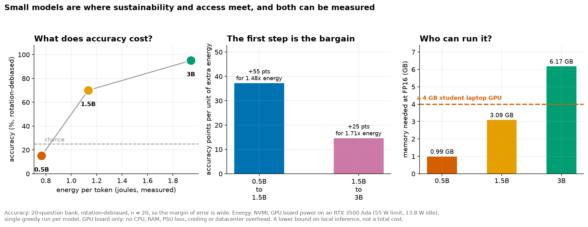
1.5 billion and 3 billion parameters. The left panel plots accuracy on the vertical axis against measured energy per token on the horizontal axis, with a grey line joining the three points. The 0.5B model sits low and left at about 15 percent accuracy and 0.77 joules per token, below a dashed grey line marked chance at 25 percent. The 1.5B model sits at about 70 percent and 1.13 joules. The 3B model sits at about 95 percent and 1.94 joules. The curve rises steeply then flattens. The middle panel is two bars showing accuracy points bought per unit of extra energy: the step from 0.5B to 1.5B reaches about 37, labelled plus 55 points for 1.48 times energy, and the step from 1.5B to 3B reaches about 15, labelled plus 25 points for 1.71 times energy. The right panel is three bars of memory needed at half precision, 0.99 gigabytes for the 0.5B, 3.09 for the 1.5B and 6.17 for the 3B, with a dashed orange horizontal line at 4 gigabytes labelled a 4 GB student laptop GPU. The first two bars sit below the line and the third rises well above it. :width: 100%
Accuracy, energy and memory for the same three models. Accuracy is from a 20-question bank
scored with the rotation-debiased procedure from Chapter 13, so its margin of error is very
wide. Energy is GPU board power measured on an RTX 3500 Ada with a 55 watt limit and a 13.8
watt idle draw, one greedy run per model. Board power only: no processor, memory, power supply
losses, cooling or datacentre overhead. Sources: lab/out/lab4_size_ladder.json and
lab/out/theme_s_energy.json.
Read the three panels in order. The left panel says accuracy climbs steeply and then flattens. The middle panel prices that flattening. The right panel says the model at the top of the curve does not fit on the hardware in question.
The mathematics
Formula 11: accuracy bought per unit of extra energy
In words. Take how many accuracy points you gained by moving to a bigger model, and divide by how many times more energy that bigger model costs per token.
The formula.
The symbols.
| Symbol | How to say it out loud | What it means |
|---|---|---|
| “bee” | the bargain: accuracy points bought per unit of extra energy | |
| “equals” | the two sides are the same number | |
| “delta” | a Greek capital letter meaning “the change in”. is the change in accuracy | |
| “ay” | accuracy, measured in percentage points from 0 to 100 | |
| “delta ay” | accuracy points gained, the bigger model’s accuracy minus the smaller model’s | |
| the fraction bar | “divided by” | divide the top by the bottom |
| “kay” | the energy multiplier: the bigger model’s joules per token divided by the smaller model’s |
The Greek letters this book uses, including , are listed with pronunciations in the Math Toolkit.
Out loud. “Bee equals delta ay over kay.” In English: accuracy points gained, divided by the energy multiplier you paid for them.
Worked, on the first step up the ladder: 0.5B to 1.5B. The rotation-debiased accuracies,
from lab/out/lab4_size_ladder.json, are 15.0 percent for the 0.5B and 70.0 percent for the
1.5B. The joules per token are 0.767069 and 1.133345.
Step 1, the accuracy gained. percentage points
Step 2, the energy multiplier.
Step 3, divide.
So accuracy points per unit of energy multiplier.
Worked again, on the second step: 1.5B to 3B. The accuracies are 70.0 and 95.0 percent. The joules per token are 1.133345 and 1.940526.
Step 1, the accuracy gained. percentage points
Step 2, the energy multiplier.
Step 3, divide.
So .
The first step bought times as much accuracy per unit of energy as the second. The first step is the bargain and the second is not, and that is a measured statement about these three models, not a general law about model scaling.
Check it. must be greater than 1 when you move to a larger model, because a larger model costs more energy per token. If comes out below 1 you have divided the two energies the wrong way round. And must be positive if the larger model scored higher; a negative would mean you paid more energy for less accuracy, which is a finding worth double-checking before publishing.
Formula 12: how much memory a model needs
In words. The memory a model needs is the number of parameters it has, times the number of bytes used to store each parameter.
The formula.
The symbols.
| Symbol | How to say it out loud | What it means |
|---|---|---|
| “capital em” | the memory the model needs, in bytes | |
| “equals” | the two sides are the same number | |
| “capital en” | how many parameters the model has. For the 0.5B model, 494,032,768 | |
| “times” | multiply | |
| “bee” | how many bytes each parameter takes. At half precision, 2 |
Half precision is the phrase for storing each of a model’s numbers in 16 bits. Sixteen bits is 2 bytes, and that is where the 2 comes from. It is also written FP16. Chapter 6 built bits and bytes up from nothing and Chapter 7 showed what happens when you store the same numbers in fewer of them.
Out loud. “Capital em equals capital en times bee.” In English: memory equals parameters times bytes per parameter.
Worked, on the 0.5B model at half precision. Here and .
Step 1, multiply. bytes
Step 2, turn bytes into gigabytes by dividing by one billion. One gigabyte here means
1,000,000,000 bytes, which is the convention lab4_size_ladder.py used when it wrote the file.
So gigabytes, which matches size_fp16_gb in lab/out/lab4_size_ladder.json
exactly.
Worked again, on the 3B model. Here and .
Step 1, multiply. bytes
Step 2, divide by one billion.
So gigabytes.
Check it. Memory must grow in proportion to parameters at a fixed precision, so doubling the parameters must double the memory. The 3B model has 6.24 times the parameters of the 0.5B and needs 6.24 times the memory, which it does. If your numbers do not scale together you have used a different for the two models without saying so.
Python
Two blocks. The first prices both steps up the size ladder using Formula 11.
# Accuracy bought per unit of extra energy, for each step up the size ladder.
print("step            accuracy gained   energy multiplier   points per multiplier")
for step_index in [0, 1]:
    smaller_key = model_keys[step_index]
    larger_key = model_keys[step_index + 1]

    accuracy_smaller = ladder_results[smaller_key]["rotation_accuracy"] * 100
    accuracy_larger = ladder_results[larger_key]["rotation_accuracy"] * 100
    accuracy_gained = accuracy_larger - accuracy_smaller

    energy_smaller = energy_results[smaller_key]["j_per_token"]
    energy_larger = energy_results[larger_key]["j_per_token"]
    energy_multiplier = energy_larger / energy_smaller

    points_per_multiplier = accuracy_gained / energy_multiplier

    step_label = smaller_key.split("-")[1] + " to " + larger_key.split("-")[1]
    print(f"{step_label:<15} {accuracy_gained:>15.0f}   {energy_multiplier:>17.4f}   {points_per_multiplier:>21.2f}")
step accuracy gained energy multiplier points per multiplier
0.5B to 1.5B 55 1.4775 37.23
1.5B to 3B 25 1.7122 14.60The first step buys 55 accuracy points for 1.4775 times the energy per token. The second buys 25 points for 1.7122 times. In the last column, 37.23 against 14.60: the first step is about two and a half times the bargain the second one is. Diminishing returns, measured on this course’s own hardware rather than asserted.
Now the second factor, in bytes.
# The access line: how much memory each model needs, against a 4 GB laptop card.
student_card_gb = 4.0

print("model                     parameters      GB at FP16   fits a 4 GB card?")
for model_key in model_keys:
    parameter_count = ladder_results[model_key]["params"]
    gigabytes_needed = ladder_results[model_key]["size_fp16_gb"]
    if gigabytes_needed <= student_card_gb:
        verdict = "yes"
    else:
        verdict = "no"
    short_name = model_key.split("/")[1]
    print(f"{short_name:<24} {parameter_count:>13,} {gigabytes_needed:>15.9f}   {verdict:>16}")
model parameters GB at FP16 fits a 4 GB card?
Qwen2.5-0.5B-Instruct 494,032,768 0.988065536 yes
Qwen2.5-1.5B-Instruct 1,543,714,304 3.087428608 yes
Qwen2.5-3B-Instruct 3,085,938,688 6.171877376 noThe last column has no middle value. The 1.5B model needs 3.087 gigabytes and a 4 gigabyte card has 0.913 gigabytes to spare. The 3B model needs 6.172 gigabytes, which is 2.172 gigabytes more than the card has, and it will not load. Not “it runs slowly”. It will not load.
The connection, stated as arithmetic
Put the two factors side by side on the same three models.
| Model | Joules per token | Accuracy points bought per unit of energy, stepping up to it | Gigabytes needed | Fits a 4 GB card |
|---|---|---|---|---|
| Qwen2.5-0.5B | 0.767 | starting point | 0.988 | yes |
| Qwen2.5-1.5B | 1.133 | 37.23 | 3.087 | yes |
| Qwen2.5-3B | 1.941 | 14.60 | 6.172 | no |
Factor one, the environmental factor, says the step from 0.5B to 1.5B is where the energy buys the most accuracy, and the step to 3B is worth less than half as much per unit of energy.
Factor two, the access factor, says the 1.5B is the largest of the three that fits on a 4 gigabyte student card. The 3B is on the other side of the access line.
Both factors select the same model, and neither one was told about the other. The energy measurement was made with a power meter on a graphics card. The memory figure was computed from a parameter count and a byte count. They came from different scripts on different days. They point at the 1.5B.
That is the connection Theme S asks students to analyse, and here it is not an argument, it is an arithmetic result you can reproduce. The reason the two factors agree is that they are both driven by parameter count. More parameters means more numbers to store, which is memory, and more multiplications per token, which is energy. Shrinking a model moves both together. That is why Chapter 7’s quantization arithmetic was simultaneously an energy argument and an access argument, and why this course puts them in the same lab.
So read the 55 points and the 25 points in Formula 11 as unpaired differences, which is the weaker of the two forms, and take the verdicts from the table above.
Chapter 12 put a 95 percent interval of 6.0 percent to 44.0 percent around a 20-question score of 25 percent, and Chapter 13 showed that the same 25 percent becomes 35 percent or 15 percent under a different defensible scoring procedure.
So the ordering 15 < 70 < 95 is probably real, and the exact values are not. The energy column was measured with a power meter and the memory column with a byte count, and both are far better measured than anything built out of accuracy. When you use this table, lean on those two columns and treat the accuracy-derived column as a sketch.
### Who is on the other side of the line

Numbers about gigabytes become a justice question when you say whose gigabytes.

California State University, Bakersfield served **10,419 students in spring 2025**, and 86
percent of them were undergraduates (<https://www.csub.edu/about/facts.shtml>, checked 19
September 2026). The Carnegie Foundation classifies CSUB as **"Opportunity Colleges and
Universities-Higher Access, Higher Earnings"**
(<https://carnegieclassifications.acenet.edu/institution/california-state-university-bakersfield/>,
checked 19 September 2026). Of the 8,792 undergraduate degree-seeking students enrolled in Fall
2024, 69 percent identified as Hispanic or Latinx, and **42 percent were first generation**,
defined as students whose parents had no post-secondary experience (NACADA Consulting,
*Academic Advising Review Report, California State University Bakersfield*, March 2025, p. 11,
<https://www.csub.edu/advising/_files/CSUB_Academic-Advising-Review-Report.pdf>).

Those figures are somebody else's, they are cited to the page, and they are not in a table with
any of this course's measurements.

Here is why they belong in a mathematics chapter. A 4 gigabyte graphics card is not a
hypothetical. It is the card in a laptop bought for a few hundred dollars, which is the machine
a lot of students in Kern County are working on. The 3B model, the one at the top of the
accuracy curve, does not load on it. The 1.5B does, with 0.913 gigabytes to spare.

So the person on the other side of the access line is not an abstraction. They are in the
library on the second floor, on the machine they could afford, and the question of which model
they can run has an answer in gigabytes that this chapter computed twice.

And here is the part worth carrying out of the course. **The cheap model and the available model
are the same model.** Choosing the small one is not a compromise between an environmental goal
and an access goal. The two goals do not trade against each other here; they point the same way,
and you can check that they do with a power meter and a parameter count.

:::{note} Three Kern County numbers this chapter wanted, and exactly why it does not have them
The argument above would be stronger with local figures on household computer ownership,
household broadband subscription, and the poverty rate in Kern County. Two routes to them were
tried on 19 and 20 September 2026, and both are worth reporting, because a dead end you can
describe precisely is more useful than one you can only complain about.

**Route one, the QuickFacts page.** <https://www.census.gov/quickfacts/kerncountycalifornia>
returned **HTTP 403** to an automated fetch. That page is built for people with browsers.

**Route two, the Census Bureau's own data API.** This is the right tool, and the variables
exist. Asking the API what the codes mean works without any credential:

- `DP02_0153PE` is "Percent, COMPUTERS AND INTERNET USE, Total households, With a computer"
- `DP02_0154PE` is "Percent, COMPUTERS AND INTERNET USE, Total households, With a broadband
  Internet subscription"
- `S1701_C03_001E` is "Estimate, Percent below poverty level, Population for whom poverty
  status is determined"

Asking it for the **values** redirects to a page headed **Missing Key**. The data endpoints now
require a free API key, and this book did not sign up for one on your behalf.

So the three figures stay **[to be measured]** here. They are not unobtainable. They are two
steps away, and both steps are yours to take.

**How to close this gap yourself**, which is a good Lab 4 warm-up. Request a free key at
<https://api.census.gov/data/key_signup.html>, then run, with your key pasted in:

```text
https://api.census.gov/data/2023/acs/acs5/profile
    ?get=NAME,DP02_0153PE,DP02_0154PE
    &for=county:029&in=state:06
    &key=YOUR_KEY_HERE
```

State 06 is California and county 029 is Kern. The poverty figure comes from the
`.../acs/acs5/subject` endpoint with `S1701_C03_001E` and the same county.

Write down the value, the vintage of the survey, and the date you fetched it, then cite all
three. A figure you looked up and dated beats a figure you remembered, every time, and it beats
one you took from a book that did not say when it was checked.
Worked example 14.2: one student, one semester, two models, one card
This runs the second half of the chapter over a single person, so the two factors land on somebody rather than on an average.
The person: one CSUB student, in the 42 percent of undergraduates who are first generation, meaning their parents had no post-secondary experience, working on a laptop with a 4 gigabyte graphics card. The course meets twice a week for 15 weeks and they generate about 500 tokens per session.
Step 1: how many tokens over the semester.
Sessions:
Tokens:
Step 2: the energy on the 1.5B model (Formula 9). Take joules per token.
joules
Step 3: the cost of that energy (Formula 10).
kilowatt-hours
cents
So the electricity for the whole semester, at the graphics card, costs about 0.13 cents. Not thirteen cents. Thirteen hundredths of one cent.
Step 4: the same student on the 3B model, for comparison. Take .
joules
kilowatt-hours
cents
The extra cost of the larger model, over a whole semester, is cents. About nine hundredths of one cent.
Step 5: the memory, on the same student’s machine (Formula 12).
1.5B: needs 3.087428608 gigabytes. The card has 4. Headroom: gigabytes. It runs.
3B: needs 6.171877376 gigabytes. Shortfall: gigabytes. It does not load.
Step 6: read the two factors against each other. The energy difference between the two models, for this student over a whole semester, is nine hundredths of a cent. The memory difference is 2.17 gigabytes, and it is the difference between a model that runs and a model that does not.
That comparison is the most important arithmetic in this chapter, and it cuts against the easy version of the environmental story. For this person, on this machine, at this scale, the electricity is not what decides anything. The hardware is. The environmental factor and the access factor point the same way, towards the smaller model, but they are not the same size: one of them is a rounding error on an electricity bill and the other one is a wall.
Step 7: what is missing, named rather than guessed. The price of the card itself is [to be measured]; this course did not survey what students paid for their machines. The energy and carbon embodied in manufacturing that card are [to be measured] for the reasons in Section 14.5. Both of those are almost certainly larger than 0.13 cents of electricity, and neither of them is in any table in this book.
Solution to Try it 14.4
1. Compare each model’s memory requirement against 8 gigabytes.
0.5B: 0.988065536 is less than 8, so it fits.
1.5B: 3.087428608 is less than 8, so it fits.
3B: 6.171877376 is less than 8, so it fits, with gigabytes to spare.
All three fit.
2. Yes, now they differ. The access factor no longer rules anything out, so it stops selecting. The environmental factor still prefers the 1.5B, because the step up to the 3B buys only 14.60 accuracy points per unit of energy against the first step’s 37.23.
3. The two factors agreed on the 4 gigabyte machine because the access line happened to fall between the 1.5B and the 3B, and that agreement is a fact about that hardware rather than a law. The honest version of the course’s claim is that both factors push in the same direction, towards smaller models, and that whether they land on exactly the same model depends on where the access line sits for the person you are talking about.
Solution to Try it 14.5
1. Using Formula 4 with :
, and .
One answer inside Group B is worth about 16.7 percentage points. Two more right answers would take Group B from 33.3 percent to 66.7 percent.
2. Group B’s accuracy is .
Margin:
Lower end:
Upper end:
The interval is , so -4.4 percent to 71.1 percent. The lower end is impossible, and the upper end reaches past 70 percent, which is close to Group A’s score. On six questions you cannot tell whether Group B is failed by this model or not.
3. Using Formula 2:
Top:
Bottom:
, which is 79.7 percent, matching the vendor’s figure.
Group B contributed 6 to a denominator of 246. Its complete failure would move the overall score by at most , which is 2.4 percentage points. The aggregate is structurally incapable of revealing a problem in Group B.
4. Something like: “Your overall figure of 79.7 percent cannot detect a problem in Group B, because Group B is 6 of 246 questions and a total failure there would move the headline by at most 2.4 percentage points. Your Group B figure of 33.3 percent also cannot detect a problem, because one answer is worth 16.7 points in a group that size and its 95 percent interval runs from below zero to above 71 percent; please re-run with at least a few hundred Group B items before we evaluate this.”
Common mistakes
Reading a subgroup row without reading its . The accuracy column and the size column have to be read together, always. A 100 percent built on two questions and a 0 percent built on one question are not results. Any table that reports subgroup accuracies without reporting subgroup sizes next to them is incomplete, and that is true whether the subgroups are statistics topics, age bands or anything else.
Treating a 100 percentage point gap as a strong finding. It is the largest gap the arithmetic allows, and it is the expected outcome when subgroups hold four questions or fewer. Section 14.4 computed that seven or more extreme subgroup rows appear about 27 percent of the time under pure guessing with no topic differences at all.
Trusting a zero-width confidence interval. When a subgroup scores 0 out of or out of , the Wald standard error comes out as exactly 0 and the interval collapses to a point. That is the formula failing, not the model being certain. Switch to the rule of three, or to the Wilson interval from Chapter 12, and say in the text which one you used.
Reporting an interval end below 0 percent or above 100 percent without comment. The assoc row’s interval ran from -0.1930 to 1.1930. Both ends are impossible. If you print that, print a sentence saying the formula has left the range where it applies.
Confusing percentage points with percent. The gap between 100 percent and 0 percent is 100 percentage points. It is not “a 100 percent difference”, and it is certainly not “infinitely better”. The Math Toolkit separates the two.
Comparing numbers that came from different procedures. This chapter’s letter counts,
{'A': 16, 'B': 3, 'C': 0, 'D': 1}, and Chapter 13’s, which that chapter printed as{'A': 16, 'D': 2, 'B': 2}with C left out because it was never chosen, are both correct and describe the same model on the same questions. They differ by one space character inside the scoring script. Check that two numbers came from the same procedure before you put them in the same sentence.Assuming a subgroup pattern is about the subgroup. Before concluding that a model is worse at probability than at study design, look for a mechanism that has nothing to do with topics. Here the mechanism was the letter A, and it explained the pattern better than any claim about statistical knowledge.
Quoting a per-run energy figure as though it were a total cost. The 0.767 joules per token figure is GPU board power only, on one laptop, for one greedy run, and about 65 percent of it is the card being switched on. It excludes training, water and embodied carbon entirely. It is a lower bound on one part of the cost.
Treating a borrowed figure as a measurement. The 27.04 cents per kilowatt-hour used in Section 14.5 is from the Energy Information Administration, covers all sectors in California in 2024, and is not a Kern County residential rate. It is labelled every time it appears and it never shares a table with a number this course measured.
Believing the access line is a matter of degree. A model that needs 6.172 gigabytes on a 4 gigabyte card does not run slowly. It does not run. Memory limits are a wall, not a slope.
What to remember
An overall benchmark score is a weighted average of the subgroups inside it, so a small group can be failed completely while the headline number looks fine. Cutting a score into subgroups is therefore something you must do on purpose, because nothing about the average will prompt you. But a subgroup score built on one to four questions is noise rather than a finding, and this chapter’s 0 percent to 100 percent spread across nine topics is exactly what pure guessing produces, with a simpler explanation available in the answer key’s two letter A’s. Running a model costs measured energy and measured memory, and on this course’s three models both point at the same choice: the 1.5B is the largest that fits a 4 gigabyte card and the step up to it buys 2.5 times as much accuracy per unit of energy as the step beyond it. A model small enough to be cheap to run is a model cheap enough for somebody to own, which is why the environmental question and the access question are one question asked twice.
Practice problems
Answers to the odd-numbered problems are in the answers appendix. Show your arithmetic. Where a problem asks for a number from a file, open the file and check.
Warm-up: can you do the arithmetic
1. A subgroup holds 5 questions and the model got 3 right. Compute its accuracy as a decimal and as a percentage.
2. A subgroup holds 8 questions. How many different accuracy values could it report? List the three smallest of them as percentages.
3. How many percentage points is one answer worth inside a subgroup of 5 questions? Of 10 questions? Of 25 questions?
4. A subgroup scores 0.60 and another scores 0.15. Compute the subgroup gap in percentage points.
5. Compute the Wald standard error for a subgroup that scored 3 out of 5. Show all four steps.
6. Using your answer to problem 5, compute the 95 percent Wald interval. Is either end outside the range 0 to 1?
7. A subgroup of 6 questions scored 0 right. Compute the rule-of-three upper limit as a percentage.
8. Compute , and .
9. A model generates 250,000 tokens at 1.133345 joules per token. Compute the total energy in joules, then in kilowatt-hours.
10. Using 27.04 cents per kilowatt-hour, compute the cost of the energy in problem 9.
11. A model has 1,543,714,304 parameters stored at 2 bytes each. Compute the memory it needs in bytes, then in gigabytes.
Practice: can you apply it
12. Open lab/out/we6_eval.json. Using the by_topic block, verify by hand that the nine
subgroup sizes add to 20 and the nine correct counts add to 5.
13. Using Formula 2 and the by_topic block, recompute the overall accuracy by hand.
Show the nine products, their sum, and the division.
14. The prob subgroup scored 0 out of 3. Compute the binomial probability of that exact result if the model’s true accuracy on every topic is 0.25. Show all five steps.
15. Compute the binomial probability that the centre subgroup, with 4 questions, scores exactly 2 right at a true accuracy of 0.25. Compare your answer with the code output in Section 14.4.
16. For each of the nine subgroups, compute , what one answer is worth. Rank the subgroups from most fragile to least.
17. The design subgroup’s Wald interval came out as . Explain in three sentences why, naming the step in Formula 6 where the collapse happens.
18. Using the energy figures in lab/out/theme_s_energy.json, compute how many joules a
section of 30 students uses if each generates 800 tokens on the 3B model. Convert to
kilowatt-hours and to cents at 27.04 cents per kilowatt-hour.
19. Compute the energy multiplier for the step from the 0.5B to the 3B model, skipping the 1.5B. Then compute for that single combined step, using the rotation accuracies of 15.0 percent and 95.0 percent. Compare it with the two separate steps and say which framing is more informative.
20. A laptop has a 6 gigabyte graphics card. Which of the course’s three models fit at half precision? Show each comparison. How much headroom is left in each case that fits?
21. Chapter 7 reported that 4-bit blockwise quantization stores a weight in 0.5625 bytes including the block scales. Recompute the 3B model’s memory at that rate using Formula 12 with , and say whether it now fits a 4 gigabyte card.
22. Explain, in four sentences and no formulas, why the aggregate score of 25 percent could not have revealed that the types subgroup scored 0 percent.
Stretch: can you reason with it
23. The chapter argues that the subgroup pattern is explained by the letter A rather than by statistical knowledge. State one piece of evidence that supports this explanation and one observation in the data that it does not fully explain. (Look at the assoc subgroup.)
24. Design a replacement question bank that would let you make a defensible claim about per-topic performance. State how many questions per topic you would need and justify the number using the rule of three. Then state what your bank would cost in energy to evaluate on the 3B model, using Formula 9 and an estimate of tokens per question that you state and justify.
25. The chapter reports that seven or more extreme subgroup rows occur about 27 percent of the time under pure guessing. Explain what that number does and does not license you to conclude. In particular, say whether it proves the model has equal skill across topics.
26. A colleague proposes reporting the subgroup gap of 100 percentage points in a paper, noting truthfully that the arithmetic is correct and the run is reproducible. Write a paragraph explaining why you would not sign that paper, and propose the specific sentence you would put in its place.
27. Section 14.6 shows the environmental factor and the access factor selecting the same model on a 4 gigabyte card, and Try it 14.4 shows them diverging on an 8 gigabyte card. Construct a third case, with a stated card size and stated model sizes, where the two factors select different models, and explain what would have to be true about the accuracy curve for that to happen.
28. This chapter marked three Kern County figures as [to be measured] after a fetch
returned HTTP 403. Write a short plan for filling them: name the source, the exact table, the
year you would report, and the sentence you would write in a lab report to make clear that the
figure is borrowed rather than measured.
29. Chapter 13 found that a 25 percentage point gap between two models could not be declared significant on 20 questions, with McNemar’s exact test returning . This chapter found subgroup gaps of 100 percentage points on 1 to 4 questions. Write one paragraph explaining, to somebody who has taken no statistics, why the larger gap is the weaker evidence.
30. The course’s thesis is that a model small enough to be environmentally cheap is a model cheap enough to be democratically available. Using only numbers from this chapter, write the strongest version of that argument in one paragraph, then write the strongest objection to it in a second paragraph. Name at least one measurement that would settle the disagreement, and say whether this course has it.
Where every number in this chapter came from
Nothing in this chapter originates anywhere else. This table is here so you can check.
Table 1:Provenance of every figure printed in Chapter 14.
| Figures | Source |
|---|---|
| 20 questions, 5 right, 25.0% overall; the nine subgroup sizes and correct counts; every per-question record, answer key letter and model answer; the Wald interval (6.0%, 44.0%) | lab/out/we6_eval.json, written by lab/we6_eval_bootstrap.py |
| The naive letter counts quoted from Chapter 13, A 16, B 2, C 0, D 2, and the accuracies 25.0%, 35.0% and 15.0% | lab/out/we6b_eval_debiased.json, written by lab/we6b_eval_debiased.py |
The letter counts {'A': 16, 'B': 3, 'C': 0, 'D': 1} used in this chapter’s diagnosis | computed in this chapter from the records block of lab/out/we6_eval.json |
| Joules per token 0.767, 1.133 and 1.941; tokens per second 27.7, 24.2 and 15.6; mean power 21.3 W, 27.4 W and 30.2 W; idle draw 13.834 W; the 55 W power limit; the 0.268 J above-idle figure | lab/out/theme_s_energy.json, written by lab/theme_s_energy.py |
| Parameter counts 494,032,768 / 1,543,714,304 / 3,085,938,688; sizes 0.988 / 3.087 / 6.172 GB at FP16; rotation-debiased accuracies 15.0% / 70.0% / 95.0% | lab/out/lab4_size_ladder.json, written by lab/lab4_size_ladder.py |
| McNemar’s exact , quoted from Chapter 13 | lab/out/we7_paired.json, written by lab/we7_paired_comparison.py |
| Every standard error, Wald interval, rule-of-three limit, binomial probability, expected extreme-topic count of 5.6953, the 0.2678 tail probability, the ratios 1.4775, 1.7122, 2.53 and 2.55, the bargain figures 37.23 and 14.60, and every energy and cost conversion | arithmetic on the files above, shown step by step in the section where it appears and computed again in the code |
| 27.04 cents per kilowatt-hour | not ours. US Energy Information Administration, California state electricity profile, average retail price across all sectors, 2024 data, release date 10 November 2025. https:// |
| 10,419 students in spring 2025, 86% undergraduate | not ours. https:// |
| “Opportunity Colleges and Universities-Higher Access, Higher Earnings” | not ours. Carnegie Classifications entry for California State University Bakersfield, https:// |
| 8,792 Fall 2024 undergraduates, 69% Hispanic/Latinx, 42% first generation | not ours. NACADA Consulting, Academic Advising Review Report, California State University Bakersfield, March 2025, p. 11. https://_research/10-csub-context-and-positioning.md section 8 rather than re-read from the PDF. Check it against page 11 before you quote it in your own work |
| Kern County household computer ownership, household broadband subscription, and poverty rate | [to be measured]. QuickFacts returned HTTP 403 on 19 September 2026; the Census data API returns “Missing Key” without a free API key, which this book did not obtain. Section 14.5 gives the exact query to run once you have one |
| Training energy, water for cooling, embodied carbon of the hardware, and the purchase price of a student graphics card | [to be measured]. See Section 14.5 and the cost model appendix |
| The 45-student section size and the 30-session semester | the course design: a section size of 45, and two sessions a week across fifteen weeks. The section size is in this course’s specification; the two-sessions-a-week structure is in this book’s reading map. The syllabus gives the 150 minutes a week but not the section size. Used as the setting for a worked example rather than as a measurement |
| The rotation standard errors 0.079844, 0.102470 and 0.048734, and the accuracy intervals computed from them | lab/out/lab4_size_ladder.json, field rotation_se, written by lab/lab4_size_ladder.py |
| The vendor table in Try it 14.5, and the shop selling coffee in Section 14.1 | made up, and labelled as such where they appear. No model produced them |