Measure your measurement - Inside the Machine: The Mathematics of Small Language Models

Chapter 13. Measure your measurement¶

What you need before this chapter¶

You need four things. Three of them you already have, and the fourth is a page you can open in another tab and keep open.

1. Chapter 11, where a model first took a test. You saw that a model’s answer has to be turned into a choice by a rule you write, and that writing that rule is a decision. If you want the mechanics again, Chapter 11 is the place.

2. Chapter 12, where a score turned out to be a random variable. You measured 25.0% on twenty questions and then measured the width of that claim: a 95% interval running from 6.0% to 44.0%. This chapter picks up where that left off. Chapter 12.

3. Arithmetic you can do on a phone. Adding, subtracting, multiplying, dividing, a few square roots, and raising a half to a small whole power. Two symbols you may not have met arrive later, “mod” in Formula 13.6 and the “choose” sign in Formula 13.11, and each one is built from nothing at the place it appears. Nothing harder than that turns up anywhere in this chapter.

4. These sections of the Math Toolkit. Each link goes to a page that starts from nothing and works arithmetic you can check. Open the ones you need when you need them.

What this chapter uses it for	Toolkit section
a letter standing for a number	Section 1, letters
$x_1$ , $x_2$ , $x_i$ : “the first one, the second one, the $i$ -th one”	Section 2, subscripts
two things written side by side, which means multiply	Section 3, multiplication
the fraction bar, which means divide	Section 4, the fraction bar
$\left(\tfrac{1}{2}\right)^5$ : a half multiplied by itself five times	Section 5, exponents
what a log-probability is	Section 8, logarithms
the square root in every standard error	Section 9, square roots
$\sum$ , which means “add these up”	Section 10, sigma notation
the standard deviation, and why it divides by one fewer	Section 10.4, standard deviation
turning 0.25 into 25% and back	Section 11, percentages
percentage points, which are not per cent	Section 11, percentage points
“5 out of 20” as a number between 0 and 1	Section 12, proportions
reading the bars in the figures	Section 13, reading a graph
what $2^5 = 32$ has to do with coin tosses	Section 18, powers of two
writing an interval as $(+5.5, +44.5)$ , and reading $p < 0.05$	Section 19, inequalities and intervals
$\Delta$ , the capital Greek D this chapter uses for a difference	Section 20, Greek letters

If you have not met the six-part shape every formula in this book arrives in, two minutes on how a formula is presented will pay for itself many times over in this chapter. There are thirteen formulas here and every one of them has the same six parts, in the same order.

The setup code¶

Run this once. Everything else in the chapter uses what it loads.

Two things are worth saying about this block before you read it. Every line has a comment, and the comments are for you, not for the computer. And nothing here runs a language model. The models were run in the lab, on the machine described in the datasets appendix, and they wrote their results into files. This chapter reads those files. That means every number you see below is a number somebody measured, and it means you can reproduce this chapter on a laptop with no graphics card in about a second.

# json reads the result files the lab wrote. Every number in this chapter comes out of one of them.
import json
# math gives us the square root, and the "choose" counting function McNemar's test needs.
import math

# The folder holding the lab's result files. Every chapter in this book uses this same folder.
results_folder = "lab/out/"

# The three scoring procedures applied to the 0.5B model. Written by lab/we6b_eval_debiased.py
three_procedures = json.load(open(results_folder + "we6b_eval_debiased.json"))

# The same question bank scored on three model sizes. Written by lab/lab4_size_ladder.py
size_ladder = json.load(open(results_folder + "lab4_size_ladder.json"))

# The 1.5B against the 3B on the same questions. Written by lab/we7_paired_comparison.py
paired_comparison = json.load(open(results_folder + "we7_paired.json"))

# How many questions are in the bank, and how many options each question has.
question_count = 20
option_count = 4

print("questions in the bank:", question_count)
print("options on each question:", option_count)
print("fields in the three-procedures file:", len(three_procedures))
print("models on the size ladder:", len(size_ladder))
print("fields in the paired-comparison file:", len(paired_comparison))

Output:

questions in the bank: 20
options on each question: 4
fields in the three-procedures file: 8
models on the size ladder: 3
fields in the paired-comparison file: 9

json.load(open(...)) opens a file and turns its contents into something Python can read. len(...) counts how many things are inside. The three files hold 8, 3 and 9 pieces of information each, which is a small amount of data to carry a whole chapter, and that is part of the point.

Where this chapter starts: a Tuesday in Bakersfield¶

It is a Tuesday in July. You step outside in Bakersfield and the air has that flat, heavy quality you know. You pull out your phone and look up the air quality for the day.

You get a number.

Now ask a harder question. What is that number a number of? Before anyone can answer, they have to tell you four other things. Which pollutant is being reported, because particle pollution and ozone are different substances measured by different instruments. Over what window, because the rule for ozone reads an eight-hour stretch and the rule for fine particles reads a full day. Measured where, because a monitor beside a freeway and a monitor in a field outside Shafter are breathing different air. And reported how, because a scale that combines several pollutants into one headline figure has to decide what to do when they disagree.

Change any one of those four decisions and the headline number changes. Nobody lied. Every version was computed correctly. The air did not change between one version and the next. What changed was the procedure, and the number belongs to the procedure at least as much as it belongs to the air.

This is not a complaint about air monitoring. Air monitoring is a serious, careful field, and the reason it publishes its rules in public documents that run to hundreds of pages is precisely that everybody in it understands the point you are about to learn. The rules are written down so that the number means something.

Now hold that thought and look at how artificial intelligence gets reported. A model scores some per cent on some benchmark. The score appears in a press release, on a leaderboard, in a purchasing decision, in a news story. The rule that produced it is usually one line in an appendix, if it appears at all.

This chapter takes one small model, one set of twenty questions, and three different rules for marking the answers. All three rules are defensible. All three appear in published research. Nothing about the model changes between them. Nothing about the questions changes.

The three numbers are 25.0%, 35.0% and 15.0%.

You are going to compute all three, work out which of them, if any, deserves to be printed, and then find out something worse: that the answer is none of them.

Where the numbers in this chapter came from

Every measured number in this chapter was produced by a script in the course repository and written to a file you can open.

The three scoring procedures: lab/we6b_eval_debiased.py wrote lab/out/we6b_eval_debiased.json.
The three model sizes: lab/lab4_size_ladder.py wrote lab/out/lab4_size_ladder.json.
The two-model comparison: lab/we7_paired_comparison.py wrote lab/out/we7_paired.json.

The question bank is twenty multiple-choice questions about general-education statistics, four options each, exactly one correct. They were written by hand for this course by your instructor. They are not a published benchmark, nobody else uses them, and they have no standing outside this book. All twenty are listed in the datasets appendix, section 3.2, with each question’s topic and its correct letter, and the four options of every question are printed in the lab script that used them, lab/we6b_eval_debiased.py. Saying that plainly matters, because the whole argument of this chapter is about how little twenty questions can settle, and that argument only works if you know exactly what you are holding.

The rule of this book is we never publish a number we did not compute. One worked example in this chapter, in Formula 13.5, uses invented log-probabilities, because small numbers are easier to check by hand, and it is labelled made up for practice where it appears. Try it 13.3, Try it 13.4 and Try it 13.5 invent their tables and their scenarios, and each says so at the top of the box. The practice problems invent theirs too, and the line above the first problem says so. Every other number on this page is a measurement, and the file it came out of is named beside it.

Learning objectives¶

By the end of this chapter you will be able to:

Explain why an evaluation score is a property of the scoring procedure as much as of the model, and give three measured numbers from one model and one question bank that prove it.
Diagnose position bias in a scoring procedure by comparing how often each option was chosen against how often each option was correct, and compute the over-choice ratio.
Apply two standard debiasing fixes, scoring the option text with length normalisation and taking a majority over cyclic rotations, and say what each one does and does not repair.
Compare two models on the same questions using a paired analysis, build the 95% interval for the difference, and say in numbers how much the pairing bought you.
Run McNemar’s exact test on a two-by-two table of paired results, interpret a p-value of 0.0625 correctly, and explain why more questions, not a stronger claim, is the fix.

This lesson at a glance¶

One model, one question bank, three defensible rules for marking it: 25.0%, 35.0%, 15.0%. A twenty percentage point spread with nothing changed but the rule.
The first rule scored exactly chance, and the reason was that it was measuring a habit. The model answered A on 16 of the 20 questions while the right answer was A twice.
Position bias is a symptom of a weak model, not a fixed tax. The gap between the naive score and the debiased score is 10 points at 0.5B, 10 points at 1.5B, and 0 points at 3B.
A 25 point gap between two models can fail to be significant. On twenty questions, with five disagreements all favouring the larger model, McNemar’s exact test returns $p = 0.0625$ .

The vocabulary of this chapter¶

Every technical term this chapter uses, defined before it is used. Read the table once now. You do not have to memorise it; you have to know it exists, so that when a word appears in a sentence you can come back and check it.

Term	What it means, in one line
scoring procedure	The complete rule for turning what a model produced into a right or a wrong.
answer extraction	The part of a scoring procedure that decides which option the model picked.
naive letter scoring	Asking which of the letter tokens A, B, C, D the model rates highest, and calling that its answer.
log-probability	The natural logarithm of a probability. A negative number. Bigger, meaning closer to zero, means more likely.
length normalisation	Dividing a total score by how many tokens it was added up over, so a long option is not punished for being long.
chance level	The score somebody would average by guessing at random. It belongs to a procedure, not to a question: with four options and one asking it is one in four, and Worked example 13.2 shows it changing when the procedure changes.
position bias	A scoring procedure rewarding an option for where it sits in the list rather than for being right.
over-choice ratio	How many times more often an option was chosen than an unbiased procedure would choose it.
cyclic rotation	Moving every option along one position and wrapping the last one round to the front.
majority vote	Asking the same question several times and keeping the answer that won most of the askings.
consistency (under rotation)	Whether the four rotations of one question all agreed with each other about whether the model was right.
debiasing gap	The naive score minus the debiased score, in percentage points.
paired comparison	Comparing two models question by question, because they answered the same questions.
unpaired comparison	Treating the two models’ scores as two separate samples, which throws the pairing away.
contingency table	A two-by-two count of how two models agreed and disagreed on the same items.
concordant pair	A question both models got right, or both got wrong.
discordant pair	A question exactly one of them got right.
standard deviation	How spread out a set of numbers is around their own average.
standard error	How much a measured number would wobble if you re-ran the whole measurement.
Wald interval	The textbook confidence interval: the measured number, plus or minus 1.96 standard errors. Built in Chapter 12, Definition 12.11, and known to be a poor fit at small sample sizes.
null hypothesis	The dull explanation a test tries to rule out: there is no real difference.
p-value	Assuming the null hypothesis is true, the chance of a result at least as lopsided as yours.
McNemar’s exact test	The significance test built for a paired yes-or-no comparison.
statistical significance	The verdict that a result is too lopsided to blame on sampling wobble, conventionally $p < 0.05$ , which is read “p is less than nought point nought five”. See the toolkit on inequalities.
failure taxonomy	A naming of the kinds of failure a model system can have, so you can say which one you are looking at.

13.1 A score belongs to a procedure, not to a model¶

Intuition¶

Think about a driving test. Two examiners, one candidate, one car, one route. Examiner A marks you on whether you completed the route safely. Examiner B marks you on a checklist of forty-three specific manoeuvres. Examiner C sits in the back, says nothing, and marks you on whether a passenger would feel comfortable.

You drove exactly the same way for all three. You could pass one and fail another. Nobody cheated. The examiners measured different things and called them all “the driving test.”

Now change one word. Instead of a candidate, a language model. Instead of a route, twenty multiple-choice questions. Instead of three examiners, three rules for reading the model’s output and deciding which option it picked.

Here is the part that catches people. A model does not “pick” an option. A language model produces a probability for every one of the 151,936 tokens it knows, for the next position in the text. That is all it produces. Nowhere in that output is there a letter circled in pencil. Somebody has to write a rule that turns 151,936 numbers into one of four letters, and that somebody is you.

The rule is not a detail. The rule is half the measurement.

There are at least three sensible rules, and all three are in use in published research:

Ask about the letter. Show the model the question with its four options and see which of the four letter tokens A, B, C and D it rates most likely to come next.
Ask about the words. Ignore the letters entirely. Score the actual text of each option, then divide by how long that option is, and take the best.
Ask four times. Move the options around the page so that every option gets a turn in every slot, ask the question once per arrangement, and keep the answer that wins the most askings.

Every one of the three is defensible. You could write a paragraph defending any of them and a reviewer would nod. They produce three different numbers on the same model and the same questions, and the distance between the highest and the lowest is twenty percentage points.

That is the whole chapter in one paragraph. The rest is working out what to do about it.

The mathematics¶

There is a formula for accuracy, and you met it in Chapter 11. This chapter writes it again with one thing added: a symbol for the procedure. That single extra symbol is the idea of the chapter made visible.

Formula 13.1: Accuracy under a scoring procedure

1. In words. To score a model, go through the questions one at a time. For each one, use your rule to decide whether the model got it right, writing down a 1 if it did and a 0 if it did not. Add up those ones and zeros, and divide by how many questions there were. The answer is the share of questions the model got right according to that rule.

2. The formula.

\hat{p}^{(g)} = \frac{1}{n} \sum_{i=1}^{n} g(M, q_i)

3. The symbols.

Symbol	How to say it out loud	What it means
$\hat{p}$	“p hat”	the accuracy you measured. A number between 0 and 1
the hat, $\hat{\phantom{p}}$	“hat”	a mark meaning “this is something we measured, not something we know for certain”
$g$	“gee”	the scoring procedure: the complete rule for marking one answer
the raised $(g)$ in $\hat{p}^{(g)}$	“under gee”	a label, not a power. It says which rule produced this accuracy
$=$	“equals”	the two sides are the same number
$\dfrac{1}{n}$	“one over en”	dividing by $n$ after adding $n$ things up is how you take an average
$\dfrac{1}{n}$ and the sum written side by side	“times”	two things written next to each other with no sign between them means multiply them. See the toolkit on multiplication
the fraction bar	“divided by”	divide the top by the bottom
$\sum_{i=1}^{n}$	“the sum from i equals one to en”	add up what follows, once for each question, starting at question 1 and stopping at question $n$ . The sign is a capital Greek S, and it is an instruction to add. See the toolkit on sigma notation
$i$	“eye”	a counter. $i = 1$ is the first question, $i = 2$ the second. See the toolkit on subscripts
$n$	“en”	how many questions there are. Here $n = 20$
$M$	“em”	the model being tested
$q_i$	“q sub i”	question number $i$
$g(M, q_i)$	“gee of em, q sub i”	what the rule $g$ gives for model $M$ on question $i$ : 1 for right, 0 for wrong

4. Out loud. “The accuracy under a procedure is one over the number of questions, times the sum, over every question, of what that procedure scored the model on that question.”

5. Worked, on the real run. The naive letter procedure marked 5 of the 20 questions right. So fifteen of the $g(M, q_i)$ values are 0 and five of them are 1.

Step 1, add up the twenty ones and zeros. Adding a 0 to a running total changes nothing, so only the five ones move the total, and the sum is the same whatever order the questions came in.

1 + 1 + 1 + 1 + 1 = 5

Step 2, divide by the number of questions.

\hat{p}^{(\text{letter})} = 5 \div 20 = 0.25

Step 3, turn that into a percentage by multiplying by 100. A percentage is a share written out of a hundred instead of out of one, so multiplying by 100 is the whole of the conversion. See the toolkit on percentages.

0.25 \times 100 = 25.0\%

Now the option-text procedure, which marked 7 right.

\hat{p}^{(\text{text})} = 7 \div 20 = 0.35, \qquad 0.35 \times 100 = 35.0\%

And the rotation procedure, which marked 3 right.

\hat{p}^{(\text{rotation})} = 3 \div 20 = 0.15, \qquad 0.15 \times 100 = 15.0\%

Step 4, the distance from the highest to the lowest.

35.0 - 15.0 = 20.0 \text{ percentage points}

6. Check it. Four checks, and they catch almost every slip anybody makes here.

Your accuracy must land between 0 and 1. If you get 1.75 you divided by the wrong thing.

Multiply your accuracy back by $n$ and you must get a whole number, because you cannot get half a question right. $0.35 \times 20 = 7$ , a whole number, so that one is sound.

None of the three numbers is finished until it carries an interval beside it. A measured accuracy is a share taken from a sample of twenty questions, so it wobbles, and Chapter 12 measured that wobble: the 25.0% comes with a 95% interval running from 6.0% to 44.0%. Write the interval down every time you write the number down. This chapter prints the three bare percentages over and over because they are the thing being argued about, and each time you read one, read the interval back onto it.

And the answer to “which is the model’s score” is not one of these three numbers. It is the question “under which procedure?”

Python¶

The three accuracies are in the file. Pull them out, turn them into counts of questions, and measure the spread.

# Pull the three accuracies out of the file, one line each.
naive_accuracy = three_procedures["naive_accuracy"]
option_text_accuracy = three_procedures["option_text_accuracy"]
rotation_accuracy = three_procedures["rotation_majority_accuracy"]

# Turn each proportion into a count of questions. "7 of 20" is easier to picture than "0.35".
naive_correct = round(naive_accuracy * question_count)
option_text_correct = round(option_text_accuracy * question_count)
rotation_correct = round(rotation_accuracy * question_count)

print("procedure 1, the letter      :", round(naive_accuracy * 100, 1), "percent  =", naive_correct, "of", question_count)
print("procedure 2, the option text :", round(option_text_accuracy * 100, 1), "percent  =", option_text_correct, "of", question_count)
print("procedure 3, four rotations  :", round(rotation_accuracy * 100, 1), "percent  =", rotation_correct, "of", question_count)

# The distance from the highest of the three to the lowest, in percentage points.
highest_accuracy = max(naive_accuracy, option_text_accuracy, rotation_accuracy)
lowest_accuracy = min(naive_accuracy, option_text_accuracy, rotation_accuracy)
spread_in_points = round((highest_accuracy - lowest_accuracy) * 100, 1)

print("highest of the three:", round(highest_accuracy * 100, 1), "percent")
print("lowest of the three :", round(lowest_accuracy * 100, 1), "percent")
print("spread              :", spread_in_points, "percentage points")

Output:

procedure 1, the letter      : 25.0 percent  = 5 of 20
procedure 2, the option text : 35.0 percent  = 7 of 20
procedure 3, four rotations  : 15.0 percent  = 3 of 20
highest of the three: 35.0 percent
lowest of the three : 15.0 percent
spread              : 20.0 percentage points

Several things in that block are worth naming, because they come back all chapter.

three_procedures["naive_accuracy"] reaches into the loaded file and takes out the value stored under the label naive_accuracy. The square brackets with a word inside them are how you ask a Python dictionary for one of its values. A dictionary is a bundle of labelled values, and it is how these result files are shaped.

round(naive_accuracy * 100, 1) does two things in one step. It multiplies the proportion by 100 to turn it into a percentage, and the 1 says keep one digit after the decimal point. Without the rounding you would sometimes see 35.000000000000004 on your screen, which is a fact about how computers store decimals and is taken apart in Chapter 6.

max(...) and min(...) give the largest and smallest of the numbers you hand them.

Now read the output slowly. Five, seven and three. Out of twenty. Those are the raw counts, and they are so small that the difference between the best and worst procedure is four questions. Four questions moved, and a reader of the headline number would come away with either “this model is worse than guessing” or “this model beats guessing by ten points.”

Both sentences would be true. Neither is a fact about the model.

Worked example 13.1: Turning a count into a percentage, and back

The option-text procedure got 7 of 20 right. Show that this is 35%, and then go the other way.

Forwards. Divide the number right by the number asked.

$7 \div 20 = 0.35$

Multiply by 100 to get a percentage.

$0.35 \times 100 = 35$ , so 35.0%.

Backwards. Somebody tells you a model scored 35% on a twenty-question bank. How many did it get right?

Turn the percentage into a decimal by dividing by 100.

$35 \div 100 = 0.35$

Multiply by the number of questions.

$0.35 \times 20 = 7$ questions.

The check. The answer to the backwards direction must be a whole number. If somebody reports 37% on a twenty-question bank, then $0.37 \times 20 = 7.4$ questions, which is impossible. Either the bank was not twenty questions or the number was rounded from something else. On a twenty-question bank the only scores that can exist are multiples of 5 percentage points: 0%, 5%, 10%, and so on up to 100%. There are exactly 21 of them. A benchmark that small cannot express “41%” at all.

13.2 A score that lands exactly on chance¶

Intuition¶

Here is a habit worth building, and it costs nothing.

When you see a score on a multiple-choice test, work out what a person who knew nothing would average, and compare. On a four-option test, somebody who closed their eyes and pointed would get about one question in four. One in four is 25%.

The naive letter procedure scored the 0.5B model at 25.0%.

Not near 25%. Not 24% or 26%. Exactly the number a coin-flipping, dice-rolling, eyes-closed guesser would average. Five questions out of twenty, which is precisely $20 \div 4$ .

There are two possible readings, and a statistician’s instinct is to check the second one first.

Reading one: the model knows nothing. That is entirely possible. It is a 494,032,768 parameter model, which is small, and the questions are about statistics. A model that knows nothing would score around chance. This reading is unremarkable and might well be true.

Reading two: the measuring instrument is broken. A thermometer that reads 20 degrees in a freezer and 20 degrees in an oven is not telling you the freezer and the oven are the same temperature. It is telling you the thermometer is not connected to anything. A scoring procedure that returns exactly the guessing rate might be measuring something that has nothing to do with whether the model knows statistics.

Reading two is worth checking first for a simple reason: if it is right, reading one has not been tested at all. You cannot conclude the model is ignorant from an instrument that is not plugged in.

A score sitting exactly on chance is not a result. It is a question. And the question is not “how much does this model know?” It is “what was that procedure actually measuring?”

This chapter answers it, and the answer is worse than you would guess.

The mathematics¶

Two small formulas, and both of them are arithmetic rather than measurement. That distinction matters and the figures in this chapter keep it visible: the chance level is drawn as a reference, never as a bar of measured data.

Formula 13.2: The chance level on a multiple-choice question

1. In words. If every question has the same number of options and exactly one of them is right, then somebody guessing at random gets one question right for every however-many options there are. The share they get right is one divided by the number of options.

2. The formula.

c = \frac{1}{k}

3. The symbols.

Symbol	How to say it out loud	What it means
$c$	“see”	the chance level: the share a random guesser averages, between 0 and 1
$=$	“equals”	the two sides are the same number
1	“one”	one correct option per question
the fraction bar	“divided by”	divide the top by the bottom. It is another way of writing a division sign. See the toolkit on the fraction bar
$k$	“kay”	how many options each question has. Here $k = 4$

4. Out loud. “The chance level is one divided by the number of options.”

5. Worked, with four options.

c = \frac{1}{4} = 1 \div 4 = 0.25

As a percentage, $0.25 \times 100 = 25.0\%$ .

And with other option counts, so the pattern is visible:

options, $k$	chance level, $c = 1/k$	as a percentage
2	$1 \div 2 = 0.5$	50.0%
3	$1 \div 3 = 0.3333$	33.3%
4	$1 \div 4 = 0.25$	25.0%
5	$1 \div 5 = 0.2$	20.0%
10	$1 \div 10 = 0.1$	10.0%

6. Check it. The chance level must fall between 0 and 1, and it must shrink as you add options, because more options means guessing gets harder. If your chance level went up when you added an option, you divided the wrong way round. And note what $c$ is not: it is not a measurement of any model. It is arithmetic about the test. No model was run to produce 0.25.

One limit on this formula, and it matters later. Formula 13.2 assumes the procedure asks each question once and takes the answer. A procedure that asks four times and requires three hits has a different and much lower chance level, and Worked example 13.2 in section 13.5 computes it. So $1 \div k$ is the chance level of a procedure, not of a question.

Formula 13.3: How many questions a guesser gets right

1. In words. Multiply the share a guesser averages by the number of questions on the test. That tells you roughly how many questions a guesser gets right.

2. The formula.

E = c \times n = \frac{n}{k}

3. The symbols.

Symbol	How to say it out loud	What it means
$E$	“ee”	the expected number of questions a guesser gets right. “Expected” here means “averages over many attempts”, not “will definitely get”
$=$	“equals”	the two sides are the same number
$c$	“see”	the chance level from Formula 13.2
$\times$	“times”	multiply
$n$	“en”	the number of questions. Here $n = 20$
$k$	“kay”	the number of options per question. Here $k = 4$
$\dfrac{n}{k}$	“en over kay”	the same thing written as one division, because $\tfrac{1}{k} \times n$ is $\tfrac{n}{k}$

4. Out loud. “The expected number right is the chance level times the number of questions, which is the number of questions divided by the number of options.”

5. Worked, on this bank.

Route one, through the chance level.

E = 0.25 \times 20 = 5

Route two, the short way.

E = \frac{20}{4} = 20 \div 4 = 5

Both routes give 5, as they must. And the naive procedure’s measured result was 5 questions right. The difference is $5 - 5 = 0$ questions.

6. Check it. $E$ can never be bigger than $n$ ; you cannot expect more right answers than there are questions. Here is the important caution, though: “expected 5” does not mean a guesser always gets exactly 5. A guesser could get 2, or 9. Chapter 12 measured that wobble for you: on twenty questions, a measured 25.0% carries a 95% interval from 6.0% to 44.0%. So the fact that the naive procedure landed exactly on 5 is a coincidence of this particular run, and the argument of this section does not depend on it being exact. Landing anywhere near chance would raise the same question.

Python¶

# Chance is arithmetic, not a measurement: one option out of four.
chance_level = 1 / option_count
print("chance level with", option_count, "options:", chance_level, "=", round(chance_level * 100, 1), "percent")

# How many of the 20 a pure guesser would get right on average.
expected_correct_by_guessing = chance_level * question_count
print("a guesser averages        :", expected_correct_by_guessing, "of", question_count)
print("the naive procedure scored:", naive_correct, "of", question_count)
print("difference                :", naive_correct - expected_correct_by_guessing, "questions")

# Say out loud what that means.
if naive_accuracy == chance_level:
    print("the naive procedure landed exactly on chance")

Output:

chance level with 4 options: 0.25 = 25.0 percent
a guesser averages        : 5.0 of 20
the naive procedure scored: 5 of 20
difference                : 0.0 questions
the naive procedure landed exactly on chance

1 / option_count is division, written with a forward slash. The single / gives a decimal answer, so 1 / 4 is 0.25 rather than 0.

The if on the second-to-last line is a condition. The indented line beneath it runs only when the thing after if is true. == with two equals signs asks “are these the same?”, which is a different question from = with one equals sign, which means “store this value under this name”. Mixing the two up is the single most common early Python mistake, and Python will tell you about it.

Read the output once more. difference: 0.0 questions. This model, marked this way, performed indistinguishably from a person who did not read the questions.

That sentence has two halves. Most people read the first half and stop. The second half, marked this way, is where the next section lives.

13.3 The diagnosis: the model was answering A¶

Intuition¶

Here is how the naive procedure works, in full, with nothing hidden.

You build a prompt. It holds the question, then the four options each on its own line with its letter in front, then the word Answer: and nothing after it. You hand that to the model and ask for the probabilities of the next token. Out come 151,936 numbers. You ignore 151,932 of them. You keep the four belonging to the tokens A, B, C and D, and whichever of those four is biggest is recorded as the model’s answer.

Now ask a question nobody normally asks. Across all twenty questions, how often did each letter win?

If the procedure were measuring knowledge, and the model had some, the answers would follow the answer key, roughly. If the model knew nothing at all and was genuinely undecided, the four letters would come up about five times each. Either way you would expect some spread.

Here is what happened.

The model answered A on 16 of the 20 questions. B twice. C never once. D twice.

And the correct answers in the bank are spread B eight times, C eight times, D twice, A twice.

Put those two lines side by side and the whole thing falls apart. The model reached for the letter A whether the question was about the mean of four numbers or about what a p-value is. The answer key rewarded A on two questions out of twenty. So the procedure gave the model credit almost by accident, on whichever questions happened to have A as the answer, plus a few lucky landings elsewhere.

That is what 25.0% was made of. Not knowledge. A habit.

And notice the direction the bias points. The letter C is the right answer on eight of the twenty questions, which is 40% of the bank, and the model chose C zero times. A procedure that can never select 40% of the correct answers has a ceiling on it that has nothing to do with what the model knows.

This has a name. When a scoring procedure rewards an option for where it sits rather than for being right, that is position bias. It is a bias in the statistical sense: a systematic push in a fixed direction, which more data does not remove. Ask this model two thousand questions instead of twenty and it will still reach for A. A bigger sample makes a random wobble smaller. It does nothing to a systematic push.

The mathematics¶

The arithmetic here is small on purpose. The point is not the difficulty; it is that nobody looks.

Formula 13.4: The over-choice ratio for one option

1. In words. Count how many times a scoring procedure landed on one particular option. Compare that with how many times it would have landed there if it had no preference between positions. Divide the first number by the second. An answer of 1 means no preference. An answer bigger than 1 means the procedure is over-choosing that option.

2. The formula.

R_j = \frac{m_j}{E} = \frac{m_j}{n/k}

3. The symbols.

Symbol	How to say it out loud	What it means
$R_j$	“R sub j”	the over-choice ratio for option $j$ . The answer
$j$	“jay”	which option we are asking about. $j = A$ , or $j = B$ , and so on
$=$	“equals”	the two sides are the same number
$m_j$	“m sub j”	how many times the procedure chose option $j$ , counted across all the questions
the fraction bar	“divided by”	divide the top by the bottom
$E$	“ee”	the expected count from Formula 13.3: $n/k$ , how often an unbiased procedure lands on each option
$n$	“en”	the number of questions, 20
$k$	“kay”	the number of options per question, 4

4. Out loud. “The over-choice ratio for an option is the number of times that option was chosen, divided by the number of times a procedure with no position preference would have chosen it.”

5. Worked, on the real run.

Step 1, work out the expected count. Every question has four options, and there are twenty questions.

E = \frac{n}{k} = \frac{20}{4} = 5

Step 2, the ratio for each letter. The chosen counts are A 16, B 2, C 0, D 2.

R_A = \frac{16}{5} = 16 \div 5 = 3.2

R_B = \frac{2}{5} = 2 \div 5 = 0.4

R_C = \frac{0}{5} = 0 \div 5 = 0.0

R_D = \frac{2}{5} = 2 \div 5 = 0.4

Step 3, read them. Option A was chosen 3.2 times more often than an unbiased procedure would. Option C was chosen 0.0 times as often, which is to say never.

Step 4, the share of all answers taken by A.

\frac{16}{20} = 16 \div 20 = 0.8, \qquad 0.8 \times 100 = 80.0\%

Four fifths of every answer this procedure produced was the letter A.

6. Check it. The chosen counts have to add to the number of questions, because every question got exactly one answer: $16 + 2 + 0 + 2 = 20$ . ✅ If yours do not add to $n$ , you mis-tallied.

And the ratios have to average to 1 across the options, because the total is fixed. Check: $3.2 + 0.4 + 0.0 + 0.4 = 4.0$ , and $4.0 \div 4 = 1.0$ . ✅ If your ratios average to something other than 1, you used the wrong expected count.

Two panels. The left panel is a horizontal bar chart of where the 494,032,768 parameters of Qwen2.5-0.5B-Instruct live, with embeddings at 28 per cent, the MLP blocks at 64 per cent and attention at 9 per cent. The right panel, which is the one this chapter needs, is a vertical bar chart of how many times the naive scoring procedure made the model choose each letter out of twenty questions: A sixteen, B two, C zero, D two, against a dashed grey reference line at five, marking what an unbiased scorer would average on each option. 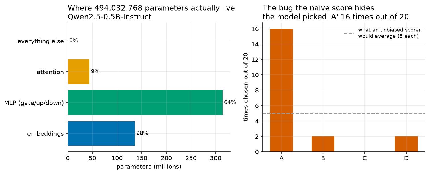— Figure 1:**The right panel is the one this chapter is about.** Each bar is one of the four options, and its height is how many times out of twenty the naive letter procedure recorded that option as the model’s answer. The dashed grey line sits at 5, which is what a procedure with no position preference would average on each option, from Formula 13.3. Option A reaches 16, which is 3.2 times the line. Option C does not appear at all, and C was the correct answer on eight of the twenty questions. The left panel belongs to Chapter 3 and is included because the two panels were drawn by the same script, `lab/make_figures.py`, from `lab/out/we3_params_quant.json` and `lab/out/we6b_eval_debiased.json`.

Python¶

# How often the naive procedure made the model 'choose' each letter.
letter_counts = three_procedures["naive_letter_counts"]

# How often each letter was the right answer. Source: _research/00-lab-verified-findings.md
# section 8, and book/appendix/datasets.md section 3.2, where all 20 answers are listed.
answer_key_counts = {"A": 2, "B": 8, "C": 8, "D": 2}

# What a scorer with no preference between positions would average on 20 questions.
expected_per_letter = question_count / option_count

print("letter   model chose   answer key   an unbiased scorer would average")
for one_letter in ["A", "B", "C", "D"]:
    print("  " + one_letter + "            " + str(letter_counts[one_letter]).rjust(2)
          + "           " + str(answer_key_counts[one_letter]).rjust(2)
          + "            " + str(expected_per_letter))

# Find the most-chosen letter with a plain loop, no shortcuts.
most_chosen_letter = "A"
for one_letter in ["A", "B", "C", "D"]:
    if letter_counts[one_letter] > letter_counts[most_chosen_letter]:
        most_chosen_letter = one_letter

biggest_count = letter_counts[most_chosen_letter]
share_of_answers = biggest_count / question_count
print("most-chosen option:", most_chosen_letter, "taken", biggest_count, "times of", question_count)
print("that is", round(share_of_answers * 100, 1), "percent of the answers")
print("an unbiased scorer would average", round(100 / option_count, 1), "percent on each option")
print("times more often than expected:", round(biggest_count / expected_per_letter, 1))

Output:

letter   model chose   answer key   an unbiased scorer would average
  A            16            2            5.0
  B             2            8            5.0
  C             0            8            5.0
  D             2            2            5.0
most-chosen option: A taken 16 times of 20
that is 80.0 percent of the answers
an unbiased scorer would average 25.0 percent on each option
times more often than expected: 3.2

The for loop repeats its indented lines once for each item in the list ["A", "B", "C", "D"]. On the first pass one_letter holds "A", on the second "B", and so on. str(...) turns a number into text so it can be glued to other text with +, and .rjust(2) pads a short piece of text on the left so the columns line up.

The second loop finds the largest of the four counts by hand. It starts by assuming A is the winner, then checks each letter in turn and moves the title whenever it finds a bigger count. There is a one-line Python shortcut for this, and this book uses the loop, because the loop is the thing you can read out loud.

Now the table. Read it column by column, not row by row.

Column two is what the procedure produced. Column three is the answer key. They have almost nothing to do with each other. The procedure’s favourite option is the key’s rarest. The key’s most common options, B and C with eight each, were chosen twice and never.

Column four is the flat line: 5.0 on every row, what a procedure with no position preference would average. The gap between column two and column four is the bias, in questions.

A last observation, and it is the one that should make you uncomfortable. If this run had been a paper, the sentence in the abstract would have been “the model performs at chance on undergraduate statistics.” That sentence is well formed, it is supported by the number, and it would survive review. It is also not supported by anything that happened, because the instrument that produced it was measuring a preference for a letter.

13.4 Fix one: score the words, not the letter¶

Intuition¶

The diagnosis suggests its own repair. The trouble came from asking about the letters. So stop asking about the letters.

Instead of “which of A, B, C or D do you rate highest”, ask something the letters play no part in. Take the prompt, and for each option in turn, stick the actual words of that option on the end and ask the model how likely that continuation was. Then take whichever option the model found most likely.

Question 1 of the bank is “The mean of 2, 4, 4, 6 is:” with options 3, 4, 5 and 6. Under this procedure the model is not being asked about the letter B. It is being asked how likely the text 4 is to follow the question. The position of 4 on the page has stopped mattering, because the position is no longer part of what you score.

There is one complication, and it is the interesting part.

Options are not all the same length. Question 14 asks what a p-value is, and one option reads “The effect size”, three words, while another reads “The probability of data this extreme if the null is true”, eleven words. Every extra token you score is another number below zero being added to the total. A longer option accumulates a worse total merely for being longer, even when the model likes every word of it.

So a procedure that took the best total would pick short options almost every time. That is a new bias, substituted for the old one.

The repair for the repair is to divide by the length. Instead of the total score for an option, take the average score per token: the total divided by how many tokens the option took. Now a long option and a short option are on the same footing, because both are being judged on how good their typical token was rather than on how many tokens they had.

That step has a name, length normalisation, and it is one line of code and a genuinely important idea. Whenever you compare totals built from different numbers of pieces, you have to decide whether you are comparing totals or averages, and the two can rank things in opposite orders.

The mathematics¶

Formula 13.5: The length-normalised score of an option

1. In words. Take one option. The model gives a log-probability for each of its tokens. Add those up, then divide by how many tokens there were. The result is the option’s typical per-token score, and it does not get worse merely because the option is long.

2. The formula.

\bar{\ell}_j = \frac{1}{L_j} \sum_{t=1}^{L_j} \ln p_{j,t}

3. The symbols.

Symbol	How to say it out loud	What it means
$\bar{\ell}_j$	“ell bar sub j”	the answer: option $j$ ’s average log-probability per token. A negative number
the bar over the $\ell$	“bar”	a mark meaning “this is an average”
$\ell$	“ell”	the letter L in a script style, used here for “log-probability”
$j$	“jay”	which option. $j = A$ , $j = B$ , and so on
$=$	“equals”	the two sides are the same number
$\dfrac{1}{L_j}$	“one over L sub j”	dividing by $L_j$ after adding $L_j$ things is how you take an average
the fraction bar	“divided by”	divide the top by the bottom. See the toolkit on the fraction bar
$\dfrac{1}{L_j}$ and the sum written side by side	“times”	two things written next to each other with no sign between them means multiply them. See the toolkit on multiplication
$L_j$	“L sub j”	how many tokens option $j$ is made of
$\sum_{t=1}^{L_j}$	“the sum from t equals one to L sub j”	add up what follows, once for each token of the option. See the toolkit on sigma notation
$t$	“tee”	a counter over the tokens of this option. $t=1$ is its first token
$\ln$	“ell en”, or “natural log”	the natural logarithm. It turns a probability between 0 and 1 into a negative number, and keeps the ranking identical. See the toolkit on logarithms
$p_{j,t}$	“p sub j comma t”	the probability the model gave to token $t$ of option $j$
$\ln p_{j,t}$	“ell en of p sub j comma t”	the log-probability of that one token. Always negative, because probabilities are below 1

4. Out loud. “The normalised score of an option is one over its number of tokens, times the sum of the log-probabilities of all its tokens.”

5. Worked. These seven numbers are made up for practice; no model produced them.

Two options. The short one is two tokens with log-probabilities -1.2 and -0.9. The long one is five tokens with log-probabilities -1.2, -0.9, -1.1, -0.8 and -1.0. That is two numbers plus five numbers, seven invented values in all.

Step 1, add up the short option’s log-probabilities.

-1.2 + (-0.9) = -2.1

Step 2, add up the long option’s.

-1.2 + (-0.9) + (-1.1) + (-0.8) + (-1.0) = -5.0

Step 3, compare the totals. -2.1 against -5.0. Since -2.1 is closer to zero, it is the larger number, so on totals the short option wins by a distance.

Step 4, divide each by its number of tokens.

\bar{\ell}_{\text{short}} = \frac{-2.1}{2} = -2.1 \div 2 = -1.05

\bar{\ell}_{\text{long}} = \frac{-5.0}{5} = -5.0 \div 5 = -1.00

Step 5, compare again. -1.00 is closer to zero than -1.05, so the long option now wins.

The ranking flipped. Nothing about the model’s opinion changed between step 3 and step 5. The only thing that changed was whether you compared totals or averages.

6. Check it. Every log-probability must be negative or zero, because every probability is between 0 and 1 and the logarithm of a number below 1 is negative. If one of yours is positive, you took the log of something that was not a probability.

The average must land between the smallest and the largest of the values you averaged. Here the long option’s values run from -1.2 to -0.8, and -1.00 sits inside that range. ✅ If your average falls outside the range of the numbers that made it, you divided by the wrong count.

Python¶

The loops below add up two short lists by hand, one number at a time, so you can see what the $\sum$ in Formula 13.5 does. Then the last two lines print the real measured result.

# A made-up example, invented for practice, to show what dividing by the length does.
# These log-probabilities are not measurements. Nothing above this line produced them.
short_option_log_probabilities = [-1.2, -0.9]
long_option_log_probabilities = [-1.2, -0.9, -1.1, -0.8, -1.0]

# Add up the short option's log-probabilities with an explicit loop.
short_option_total = 0.0
for one_value in short_option_log_probabilities:
    short_option_total = short_option_total + one_value

# Add up the long option's log-probabilities the same way.
long_option_total = 0.0
for one_value in long_option_log_probabilities:
    long_option_total = long_option_total + one_value

print("short option, total    :", round(short_option_total, 4), "over", len(short_option_log_probabilities), "tokens")
print("long option, total     :", round(long_option_total, 4), "over", len(long_option_log_probabilities), "tokens")
print("short option, per token:", round(short_option_total / len(short_option_log_probabilities), 4))
print("long option, per token :", round(long_option_total / len(long_option_log_probabilities), 4))

# Now the real measurement, from the file.
option_text_counts = three_procedures["option_text_counts"]
print("real run, option-text procedure:", round(option_text_accuracy * 100, 1), "percent")
print("real run, which positions it chose:", option_text_counts)

Output:

short option, total    : -2.1 over 2 tokens
long option, total     : -5.0 over 5 tokens
short option, per token: -1.05
long option, per token : -1.0
real run, option-text procedure: 35.0 percent
real run, which positions it chose: {'A': 7, 'B': 11, 'C': 2, 'D': 0}

short_option_total = 0.0 sets up an empty running total before the loop starts. Then short_option_total = short_option_total + one_value adds the next number to it. Read that line right to left: take what the total currently holds, add the new value, store the answer back under the same name. A loop that does this is an accumulator, and it is how every $\sum$ in this book is carried out in code. len(...) counts how many items are in a list.

Now the measured result, and it comes in two halves.

The good half. The score went from 25.0% to 35.0%. Seven questions out of twenty instead of five. That is two more questions, and it is ten percentage points above the chance level.

The half nobody prints. Look at where this procedure’s answers landed: A seven times, B eleven times, C twice, D never. Against an answer key of A two, B eight, C eight, D two.

It is a different bias. It is not a smaller one.

This procedure now over-chooses B, by a ratio of $11 \div 5 = 2.2$ . It still barely touches C, choosing it twice where the key rewards it eight times. It never once selects D. An unbiased procedure would land on each option about five times; this one produced 7, 11, 2 and 0.

So the honest report on fix one is: the score improved, and the instrument is still bent. It is bent in a new direction, which makes it harder to notice, because 35% does not sit suspiciously on the chance line the way 25% did.

That is the most dangerous kind of broken instrument: the one whose reading looks plausible.

13.5 Fix two: move the options around¶

Intuition¶

The second fix goes at the problem from the other end, and it is the more powerful of the two.

If you suspect the model is answering based on where an option sits, then move the options and see whether its answer follows. That is all. It is exactly what a careful teacher does when they suspect a student copied: they hand out the same test with the questions in a different order.

Here is the procedure in full. Take one question. Ask it four times. On the first asking, leave the options where they are. On the second, move every option up one place and wrap the top one round to the bottom, so what was option B is now option A. On the third, move them again. On the fourth, again. After four moves every option has occupied every position exactly once. That sliding-and-wrapping move is called a cyclic rotation.

Each time, you write down whether the model landed on the correct option, wherever the correct option happens to be sitting now. Then you take the majority: if the model was right on at least three of the four askings, the question counts as correct.

A model that knows an answer will follow that answer around the page. If it knows the mean of 2, 4, 4 and 6 is 4, it should select 4 whether 4 is sitting in slot A, B, C or D. A model that is reaching for a position will be right exactly once in four, because the correct option passes through its favourite slot exactly once during the rotation.

Read that last sentence again, because it is the sharp edge of this section. A model that always answers A scores one out of four on every single question under rotation, and one out of four is below the three-out-of-four majority, so it fails every question. Rotation does not soften position bias. It removes the reward for it entirely.

Applied to all twenty questions, the score came out at 15.0%. Three questions of twenty. Below the naive 25.0%. Below the option-text 35.0%.

Here is where you have to be careful, and it is the chapter’s own lesson turned back on the chapter. It is tempting to write “and 15.0% is below the chance level of 25%.” That sentence is wrong. The 25% chance level belongs to a procedure that asks each question once. This procedure asks each question four times and demands at least three hits, which is a much harder target for a guesser. A guesser facing this rule averages about 5.1%, not 25%, and Worked example 13.2 does that arithmetic in full. So 15.0% is in fact above chance for the procedure that produced it.

Changing the rule changed the chance level too. A chance level is a property of a procedure, in exactly the way a score is, and comparing a score from one procedure against a chance level computed for another is the same mistake in a smaller costume.

And the second number this procedure produces is the one that ends the argument. Of the twenty questions, the four rotations agreed with each other on exactly one.

The mathematics¶

Two formulas and one worked example. The first formula says where the correct answer moves to. The second is the punchline. The worked example settles what a guesser would score under this rule, which is the line the 15.0% has to be read against.

Formula 13.6: Where the correct answer sits after a rotation

1. In words. When you slide all the options up by some number of places and wrap the ones that fall off the top around to the bottom, the correct answer moves up by the same number of places, and it wraps around too. To find where it landed, subtract the number of places you slid, and if the answer goes below zero, add the number of options back on.

2. The formula.

g_r = (g - r) \bmod k

3. The symbols.

Symbol	How to say it out loud	What it means
$g_r$	“g sub r”	the answer: which position the correct option occupies after rotation $r$
$g$	“gee”	which position the correct option started in. Counting from 0, so position 0 is option A, position 1 is option B, position 2 is C, position 3 is D. This is not the $g$ of Formula 13.1, which stood for a scoring procedure. A letter gets re-used for a new job now and then, and when this book does that it says so
$r$	“arr”	how many places you slid the options. $r = 0$ means no slide
$=$	“equals”	the two sides are the same number
$-$	“minus”	subtract
the round brackets, $(\;)$	“bracket, close bracket”	do what is inside them first. So $(g - r) \bmod k$ means subtract first, then take the remainder
$\bmod$	“mod”, short for “modulo”	the remainder after dividing. It is what makes the wrapping happen
$k$	“kay”	how many options there are, 4

A note on “mod”, which is one of the two unfamiliar symbols in this chapter. The other is the “choose” sign in Formula 13.11, and it gets the same treatment when it arrives. $\bmod$ means “take the remainder after dividing”. So $7 \bmod 4 = 3$ , because 7 divided by 4 is 1 with 3 left over. It is the arithmetic of a clock face: five hours after ten o’clock is three o’clock, because $15 \bmod 12 = 3$ . When the number underneath is negative, keep adding $k$ until it is not: $-1 \bmod 4 = 3$ , because $-1 + 4 = 3$ .

4. Out loud. “The correct position after a rotation is the starting position minus the rotation number, with the remainder taken after dividing by the number of options.”

5. Worked, on question 1 of the bank. The question is “The mean of 2, 4, 4, 6 is:” and the options are 3, 4, 5, 6. The correct answer is 4, sitting in position 1, which is option B.

Rotation $r = 0$ . No slide.

g_0 = (1 - 0) \bmod 4 = 1 \bmod 4 = 1 \rightarrow \text{option B}

Rotation $r = 1$ . The options become 4, 5, 6, 3.

g_1 = (1 - 1) \bmod 4 = 0 \bmod 4 = 0 \rightarrow \text{option A}

Rotation $r = 2$ . The options become 5, 6, 3, 4.

g_2 = (1 - 2) \bmod 4 = (-1) \bmod 4 = 3 \rightarrow \text{option D}

That third line is where the wrapping shows. $1 - 2 = -1$ , and $-1 + 4 = 3$ , so the correct answer is now option D.

Rotation $r = 3$ . The options become 6, 3, 4, 5.

g_3 = (1 - 3) \bmod 4 = (-2) \bmod 4 = 2 \rightarrow \text{option C}

6. Check it. Across the four rotations the correct answer must visit all four positions exactly once. Here it visited B, A, D, C. ✅ Every letter appears once. If one letter appears twice, you have a mistake in the mod arithmetic, and the usual cause is not adding $k$ back on when the subtraction went negative.

Formula 13.7: The consistency rate under rotation

1. In words. Count how many questions the four rotations agreed on, meaning the model was right all four times or wrong all four times. Divide by the number of questions. That gives you the share of questions where the model behaved the same way no matter where the options sat.

2. The formula.

\hat{c} = \frac{u}{n}

3. The symbols.

Symbol	How to say it out loud	What it means
$\hat{c}$	“c hat”	the answer: the consistency rate, between 0 and 1. This is not the $c$ of Formula 13.2, which was the chance level. The hat is the clue: this one was measured
the hat	“hat”	a mark meaning “measured, not known for certain”
$=$	“equals”	the two sides are the same number
$u$	“you”	how many questions the four rotations agreed on: right four times, or wrong four times
the fraction bar	“divided by”	divide the top by the bottom
$n$	“en”	the number of questions, 20

4. Out loud. “The consistency rate is the number of questions the rotations agreed on, divided by the number of questions.”

5. Worked, on the real run. The lab measured $u = 1$ out of $n = 20$ .

\hat{c} = \frac{1}{20} = 1 \div 20 = 0.05, \qquad 0.05 \times 100 = 5.0\%

Now work out what a position-locked model would score, so you have something to compare against. Suppose a model always picks position A, whatever the question says. On each question the correct answer passes through position A exactly once in the four rotations, so the model is right once and wrong three times. That is neither four-out-of-four nor zero-out-of-four, so the rotations disagree, and the question is not consistent.

\hat{c}_{\text{always-A}} = \frac{0}{20} = 0.0

And a model that genuinely knows the material is right on all four rotations of every question it knows, so those questions are consistent.

So the consistency rate runs from 0, for a model that is purely following positions, up towards 1, for a model that is actually reading the options. The measured 0.05 sits almost at the bottom of that range.

6. Check it. $u$ cannot exceed $n$ , so $\hat{c}$ cannot exceed 1. And here is a check on your understanding rather than your arithmetic: a low consistency rate is not the same as a low score. A model could be consistently wrong on every question, always picking the same incorrect option, and score 0% with a consistency rate of 1.0. That would tell you it had a firm, wrong opinion. A consistency rate near zero tells you something different and worse: the answers are not opinions at all.

Worked example 13.2: The chance level of the rotation procedure

Formula 13.2 said the chance level with four options is $1 \div 4 = 0.25$ . That was for a procedure that asks each question once. The rotation procedure asks four times and requires at least three hits. Work out what a guesser averages under that rule.

Step 1, the chance of one asking. Four options, one right, so $1 \div 4 = 0.25$ , and the chance of missing is $1 - 0.25 = 0.75$ .

Step 2, list the outcomes that count as correct. The rule needs 3 or 4 hits out of 4. So there are two outcomes to add up: exactly 3 hits, and exactly 4 hits.

Step 3, exactly 4 hits. All four askings have to land. Multiply 0.25 by itself four times.

0.25 \times 0.25 = 0.0625

0.0625 \times 0.25 = 0.015625

0.015625 \times 0.25 = 0.00390625

Step 4, exactly 3 hits. Three askings land and one misses, which is $0.25 \times 0.25 \times 0.25 \times 0.75$ .

0.25 \times 0.25 \times 0.25 = 0.015625

0.015625 \times 0.75 = 0.01171875

But the miss could be any one of the four askings, so there are four ways this can happen. That count is the “choose” sign of Formula 13.11 doing a small job: $\binom{4}{3} = 4$ .

4 \times 0.01171875 = 0.046875

Step 5, add the two outcomes.

0.046875 + 0.00390625 = 0.05078125

Step 6, as a percentage.

0.05078125 \times 100 = 5.078125\%, \text{ which rounds to } 5.1\%

The check. The answer has to be smaller than the single-asking chance level of 25%, because the rule asks for three hits where before it asked for one, and asking for more cannot make guessing easier. And 5.1% is smaller than 25%. ✅ A second check: written as a fraction the answer is $13 \div 256$ , and $256 = 2^8$ , which is a whole number of halvings, so the arithmetic is exact rather than rounded.

One assumption, stated. Steps 3 and 4 multiply the four askings together, and multiplying probabilities like that assumes the four askings do not influence each other. For a guesser that is true. For a real model it is not: a model with a habit will lean the same way every time. So 5.1% is the chance level for guessing, which is what a chance level is for, and it is not a prediction about any particular model.

What it means. The measured 15.0% is about three times the 5.1% a guesser would average under this rule. Read against its own chance level, the rotation score is not a chance result. It is a low score, from a weak model, on a procedure that no longer pays for a position habit. The rotation procedure is also the one the two-model comparison in section 13.7 runs on, so knowing where its chance line sits is worth the two minutes.

Read the definition of a metric before you quote it

The consistency count in lab/out/we6b_eval_debiased.json counts a question as consistent when the four rotations agreed on the verdict: right all four times, or wrong all four times. You can read that in the script, lab/we6b_eval_debiased.py, in the line if sum(votes) in (0, 4).

That is subtly different from “gave the same answer all four times”. A model could be wrong four times while giving four different wrong answers, and this measure would count it as consistent.

The distinction does not change the conclusion here, because of the argument worked in Formula 13.7: a model locked onto one position is right exactly once in four and therefore counts as inconsistent under this measure. So a consistency of 1 out of 20 is, if anything, harsher on the model than the looser phrase would be.

This point belongs in a chapter about measuring your measurement, and it applies to this book as much as to anyone else’s. A metric is a procedure. Read its definition before you quote its number, including when the number is ours.

Python¶

# Question 1 of the bank, with its four options in their printed order.
option_list = ["3", "4", "5", "6"]
letter_list = ["A", "B", "C", "D"]

# The right answer is 4, which sits in position 1, because Python counts from 0.
correct_position = 1

for rotation_number in range(option_count):
    # Rotate left: take everything from rotation_number onward, then everything before it.
    rotated_options = option_list[rotation_number:] + option_list[:rotation_number]
    # Work out where the right answer has moved to. The % sign is remainder after division.
    new_correct_position = (correct_position - rotation_number) % option_count
    print("rotation", rotation_number, rotated_options,
          " the right answer is now option", letter_list[new_correct_position])

# The two measured results of doing this to all 20 questions.
consistent_questions = three_procedures["fully_consistent_questions"]
print("score under majority-of-four-rotations:", round(rotation_accuracy * 100, 1), "percent")
print("questions where all four rotations agreed:", consistent_questions, "of", question_count)
print("that is", round(100 * consistent_questions / question_count, 1), "percent consistent")

Output:

rotation 0 ['3', '4', '5', '6']  the right answer is now option B
rotation 1 ['4', '5', '6', '3']  the right answer is now option A
rotation 2 ['5', '6', '3', '4']  the right answer is now option D
rotation 3 ['6', '3', '4', '5']  the right answer is now option C
score under majority-of-four-rotations: 15.0 percent
questions where all four rotations agreed: 1 of 20
that is 5.0 percent consistent

Three pieces of Python are new here.

option_list[rotation_number:] takes a slice of a list: everything from that position to the end. option_list[:rotation_number] takes everything before that position. Gluing the two together with + performs the rotation. On the second pass, rotation_number is 1, so the first slice is ['4','5','6'], the second is ['3'], and together they make ['4','5','6','3'].

% between two whole numbers is the remainder after division, which is the $\bmod$ from Formula 13.6. In Python, (1 - 2) % 4 gives 3, with the wrapping already handled for you.

range(option_count) produces the numbers 0, 1, 2, 3. It stops before the number you give it, which catches everybody once.

Now the output. The first four lines show the correct answer visiting B, A, D and C, one position per rotation, exactly as Formula 13.6 predicted.

The last three lines are the real result, and the middle one is the most important number in this chapter.

One question out of twenty.

On nineteen of the twenty questions, moving the options around changed whether the model was right. Its answers were not opinions about statistics that happened to be wrong. They were responses to the layout of the page.

At this point you have three numbers, 25.0%, 35.0% and 15.0%, and you could defend any one of them in writing. But the consistency count tells you what the honest report is, and it is not a number at all. It is a sentence: this model does not know this material, and a single figure should not have been printed.

That sentence is worth more than any of the three percentages. It is also the sentence that never appears on a leaderboard.

The simulation¶

Everything in sections 13.1 through 13.5 is in the page below, and you can move between the two views with the slider. View 0 puts the three procedures side by side against the chance level. View 1 is the diagnosis: for each letter, how often the model chose it against how often it was the right answer.

Try it 13.1: Predict before you look

Before you move the slider, answer these three on paper.

A model that had genuinely learned this material would produce a letter-count spread close to which four numbers?
If a scoring procedure chose option C zero times out of twenty, what is the highest score it could possibly reach on this bank?
The naive procedure scored 25.0% and the rotation procedure scored 15.0%. Which of the two is closer to the truth about what this model knows, and why is that a trick question?

A bar chart with three bars showing reported accuracy as a percentage for three scoring procedures applied to the same model on the same twenty questions. Scoring by the log-probability of the letter gives 25 per cent. Scoring by the log-probability of the option text gives 35 per cent. Majority over four rotations gives 15 per cent. A dashed horizontal line marks the chance level at 25 per cent, which the first bar sits exactly on. 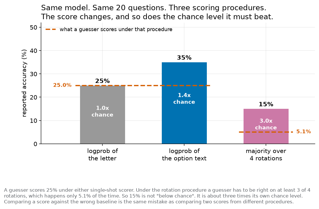— Figure 2:**One model, one question bank, three defensible procedures.** Each bar is `Qwen2.5-0.5B-Instruct` scored on the same twenty statistics questions. The only thing that differs between the bars is the rule used to decide which option the model picked. The dashed line at 25% is the chance level from Formula 13.2, and it is arithmetic rather than a measurement: with four options, guessing gets one in four. The first bar lands exactly on it. Read that line against the first two bars only. It is the chance level of a procedure that asks each question once, and both of those do. The third bar comes from a rule that asks four times and requires three hits, whose chance level is 5.1% rather than 25%, worked out in Worked example 13.2. Drawn by `lab/make_figures.py` from `lab/out/we6b_eval_debiased.json`.

13.6 Position bias is a symptom of weakness, not a fixed tax¶

Intuition¶

A reasonable reader reaches this point and draws the wrong conclusion. It goes like this: “Position bias inflates naive scores. So every naive score is inflated by roughly ten points, and I should mentally subtract ten from anything I read.”

That would be tidy. It is also wrong, and the evidence against it is in the course lab.

The same twenty questions were put to three models from the same family: the 0.5B, the 1.5B and the 3B. Same questions, same prompts, same code, same machine. Size is the only thing that changes, which makes this a controlled experiment in the ordinary scientific sense. Each model was scored twice, once by the naive letter procedure and once by the rotation procedure. The distance between those two scores is what this section calls the debiasing gap.

Here is what the gap did as the models got bigger.

At 0.5B, the gap is 10 points: 25.0% naive, 15.0% rotated. At 1.5B, the gap is 10 points: 80.0% naive, 70.0% rotated. At 3B, the gap is 0 points: 95.0% naive, 95.0% rotated.

The largest model’s score does not move when you take the position bias away. Rotating the options changes nothing, because it was never answering on position in the first place.

And look at how the 3B distributed its first-pick answers: B eight times, C seven, D twice, A three times. Now put the answer key beside it: B eight, C eight, D two, A two. Those two lines are nearly the same line. The model is not picking positions. It is picking answers, and the answers happen to sit where they sit.

The consistency counts tell the same story from the other side. Under four rotations, the number of questions where all four rotations agreed on the verdict went 1, then 13, then 18, out of twenty.

So position bias is not a tax levied on all benchmark scores. It is a symptom that appears when a model does not know the answer. When a model has no view about which option is right, the only thing left to break the tie is a habit, and a preference for the letter A is such a habit. When the model does have a view, the habit is overridden and the bias vanishes on its own.

That reframes the diagnosis in section 13.3. The 16-out-of-20 A count was not a separate defect sitting alongside a weak model. It was what a weak model looks like when you score it that way.

The mathematics¶

Formula 13.8: The debiasing gap

1. In words. Score the model twice, once with the naive procedure and once with a procedure that removes the position preference. Subtract the second score from the first. A large answer means the naive score was propped up by something other than knowledge. An answer of zero means the position preference was not doing any work.

2. The formula.

\Delta = \hat{p}^{(\text{naive})} - \hat{p}^{(\text{rot})}

3. The symbols.

Symbol	How to say it out loud	What it means
$\Delta$	“delta”	a capital Greek D. In this book it marks a difference between two things. Here, the answer. See the toolkit on Greek letters
$=$	“equals”	the two sides are the same number
$\hat{p}^{(\text{naive})}$	“p hat under naive”	the accuracy under the naive letter procedure
$\hat{p}^{(\text{rot})}$	“p hat under rot”	the accuracy under the rotation procedure
the raised label in brackets	“under”	a label naming a procedure, never a power
$-$	“minus”	subtract the second from the first

4. Out loud. “The debiasing gap is the naive accuracy minus the rotation accuracy.”

5. Worked, on all three models.

The 0.5B model.

\Delta = 0.25 - 0.15 = 0.10, \qquad 0.10 \times 100 = 10.0 \text{ percentage points}

The 1.5B model.

\Delta = 0.80 - 0.70 = 0.10, \qquad 0.10 \times 100 = 10.0 \text{ percentage points}

The 3B model.

\Delta = 0.95 - 0.95 = 0.00, \qquad 0.00 \times 100 = 0.0 \text{ percentage points}

6. Check it. $\Delta$ can be negative, and that is informative rather than an error: it would mean the debiased procedure scored higher, which happens when a model’s position habit was pushing it away from correct answers rather than towards them.

The honest caution, and it belongs here rather than in a footnote. Each of these numbers comes from twenty questions. A difference of one question is 5 percentage points on a bank this size. The file lab/out/lab4_size_ladder.json carries a measured standard error for each rotation score, and they are large: 0.0798 at 0.5B, 0.1025 at 1.5B and 0.0487 at 3B, which as percentage points is 8.0, 10.2 and 4.9. Every score in this section should be read with a wobble of about that size around it. The 0-point gap at 3B is built on the model getting 19 of 20 both times. If the 3B had missed one extra question under rotation, the gap would read 5 points instead of 0. So the shape of the ladder, large gap at the bottom and no gap at the top, is the finding here. The precise gap values are far less certain than printing them to one decimal place suggests, and Chapter 12 is the chapter that taught you why.

Python¶

print("model                          naive   rotation    gap   consistent   first-pick spread")
for model_name in size_ladder:
    one_model = size_ladder[model_name]
    naive_for_this_model = one_model["naive_accuracy"]
    rotation_for_this_model = one_model["rotation_accuracy"]
    # The debiasing gap: how much the naive number fell when the bias was taken away.
    gap_in_points = round((naive_for_this_model - rotation_for_this_model) * 100, 1)
    short_name = model_name.split("/")[1]
    print(short_name.ljust(30),
          str(round(naive_for_this_model * 100, 1)).rjust(5),
          str(round(rotation_for_this_model * 100, 1)).rjust(9),
          str(gap_in_points).rjust(7),
          (str(one_model["consistent"]) + " of 20").rjust(12),
          "  ", one_model["first_pick_spread"])

print("the answer key spread, for comparison:", answer_key_counts)

Output:

model                          naive   rotation    gap   consistent   first-pick spread
Qwen2.5-0.5B-Instruct           25.0      15.0    10.0      1 of 20    {'A': 16, 'D': 2, 'B': 2}
Qwen2.5-1.5B-Instruct           80.0      70.0    10.0     13 of 20    {'C': 7, 'B': 7, 'D': 2, 'A': 4}
Qwen2.5-3B-Instruct             95.0      95.0     0.0     18 of 20    {'B': 8, 'C': 7, 'D': 2, 'A': 3}
the answer key spread, for comparison: {'A': 2, 'B': 8, 'C': 8, 'D': 2}

for model_name in size_ladder walks through the labels in the loaded dictionary, one per model. model_name.split("/")[1] cuts the text Qwen/Qwen2.5-3B-Instruct at the slash and keeps the second piece, so the table is readable. .ljust(30) and .rjust(5) pad text on the right or the left so the columns line up.

Read this table from the bottom up.

The last row and the last line. {'B': 8, 'C': 7, 'D': 2, 'A': 3} against the key’s {'A': 2, 'B': 8, 'C': 8, 'D': 2}. B matches exactly at 8. C is off by one, 7 against 8. D matches exactly at 2. A is off by one, 3 against 2. A model that is reading the options produces an answer spread that looks like the answer key, and this one does.

The first row. {'A': 16, 'D': 2, 'B': 2}, with C missing entirely because it was never chosen. A model that is not reading the options produces a spread that looks like a habit.

The consistent column. 1, then 13, then 18, out of twenty. These are the questions where all four rotations agreed on the verdict, in the precise sense set out in section 13.5. This is the cleanest single column in the table. It rises with size and it rises fast, and it is the column that tells you whether the answers mean anything before you look at any score.

The gap column. 10.0, 10.0, 0.0. The gap does not fall smoothly. It holds at ten points across a threefold increase in size and then goes to zero. Twenty questions is nowhere near enough data to say anything about the shape of that fall, and this book will not pretend otherwise. What the column does support is the qualitative claim: the gap is present when the model is weak and absent when it is strong.

Try it 13.2: Reading the ladder

Using only the printed table:

The 1.5B model chose A four times out of twenty. Compute its over-choice ratio for A, using Formula 13.4.
The 0.5B chose A sixteen times. Compute the same ratio, and say how many times larger it is.
Somebody claims “the 1.5B still has a position bias, because its naive and rotation scores differ by 10 points.” Is the letter spread consistent with that claim?

13.7 Comparing two models: the wrong way, then the right way¶

Intuition¶

Everything so far has been about one model. Almost every real question is about two.

Should the department install the 1.5B or the 3B? The 3B is more accurate and costs more energy per token, a trade-off Chapter 7 measured. But before that trade-off is even worth discussing, somebody has to establish that the 3B is actually better, and by how much, and with what certainty.

The two models sat the same twenty questions, under the same rotation-debiased procedure.

Qwen2.5-1.5B-Instruct scored 14 of 20, which is 70.0%.
Qwen2.5-3B-Instruct scored 19 of 20, which is 95.0%.
The gap is 25.0 percentage points.

Now, how uncertain is that 25-point gap? There are two ways to work it out and they differ in one assumption.

The unpaired way treats the two results as two separate surveys. You worked out the wobble for one model’s score in Chapter 12; do that twice and combine. This is the standard formula for comparing two proportions and it is in every introductory statistics book.

It is also the wrong tool here, and the reason is a single sentence: the two models answered the same questions.

Think about what that means. Question 5 of the bank is hard, or it is easy, and it is exactly as hard or as easy for both models. That shared difficulty is not noise to be averaged away. It is information you paid for by using the same bank, and the unpaired formula throws it in the bin.

The paired way keeps it. Go through the questions one at a time and write down, for each one, what the 3B did minus what the 1.5B did. That difference can only be three things: +1 if the 3B got it right and the 1.5B did not, -1 if the reverse, and 0 if they did the same thing.

Then average those twenty differences. The average comes out to exactly the same 25 points, as it always must. But the spread of the differences is smaller than the spread of the two separate scores, because every question the models agreed on contributes a 0, and zeros pull a spread down.

Smaller spread, smaller standard error, narrower interval. Same data, better answer, no extra questions asked.

The mathematics¶

Two formulas here. The first is the unpaired standard error, shown so you can see what it costs. The second is the paired one.

Formula 13.9: The unpaired standard error of a difference

1. In words. Work out the wobble in each model’s score separately. Add the two wobbles together, inside the square root, and take the square root of the total. This is how you would do it if the two models had sat two different tests.

2. The formula.

SE_{\text{unpaired}} = \sqrt{\frac{\hat{p}_A(1 - \hat{p}_A)}{n} + \frac{\hat{p}_B(1 - \hat{p}_B)}{n}}

3. The symbols.

Symbol	How to say it out loud	What it means
$SE_{\text{unpaired}}$	“ess ee unpaired”	the answer: how much the measured gap would wobble on a re-run, computed the wrong way for this data
$=$	“equals”	the two sides are the same number
$\sqrt{\phantom{x}}$	“the square root of”	the number which, multiplied by itself, gives what is underneath. $\sqrt{9} = 3$ because $3 \times 3 = 9$ . It covers the whole sum here, not one piece. See the toolkit on square roots
$\hat{p}_A$	“p hat sub A”	model A’s accuracy. Here the 1.5B, at 0.70. From this formula onwards, $A$ and $B$ name the two models. They are no longer the options A and B on a question
$\hat{p}_B$	“p hat sub B”	model B’s accuracy. Here the 3B, at 0.95
$1 - \hat{p}_A$	“one minus p hat sub A”	the share model A got wrong. Here $1 - 0.70 = 0.30$
$1 - \hat{p}_B$	“one minus p hat sub B”	the share model B got wrong. Here $1 - 0.95 = 0.05$
$\times$ , written as juxtaposition	“times”	$\hat{p}_A(1 - \hat{p}_A)$ means multiply those two together. See the toolkit on multiplication
the fraction bars	“divided by”	divide each top by its own bottom
$n$	“en”	the number of questions, 20 for both
$+$	“plus”	add the two pieces together, inside the square root

4. Out loud. “The unpaired standard error is the square root of: model A’s accuracy times one minus it, divided by the number of questions, plus model B’s accuracy times one minus it, divided by the number of questions.”

5. Worked, step by step.

Step 1, model A’s piece, with $\hat{p}_A = 0.70$ .

$1 - 0.70 = 0.30$

$0.70 \times 0.30 = 0.21$

$0.21 \div 20 = 0.010500$

Step 2, model B’s piece, with $\hat{p}_B = 0.95$ .

$1 - 0.95 = 0.05$

$0.95 \times 0.05 = 0.0475$

$0.0475 \div 20 = 0.002375$

Step 3, add the two pieces.

$0.010500 + 0.002375 = 0.012875$

Step 4, take the square root.

$\sqrt{0.012875} = 0.113468$

Step 5, build the 95% interval around the measured gap of 0.25. The multiplier 1.96 is the one Chapter 12 introduced for 95%.

$1.96 \times 0.113468 = 0.222397$

$0.25 - 0.222397 = 0.027603$

$0.25 + 0.222397 = 0.472397$

Those two numbers are shares, between 0 and 1. Turn each into percentage points by multiplying by 100, the same move as in Worked example 13.1.

$0.027603 \times 100 = 2.7603$ , which rounds to 2.8

$0.472397 \times 100 = 47.2397$ , which rounds to 47.2

As percentage points, the interval is $(+2.8, +47.2)$ . Two numbers inside round brackets with a comma between them is how this book writes an interval: the first number is the bottom end, the second is the top end, and the claim is that the true gap sits somewhere between them. See the toolkit on inequalities and intervals.

6. Check it. The whole thing lives under one square root. A common slip is taking the root of each piece and then adding, which gives $\sqrt{0.0105} + \sqrt{0.002375} = 0.1025 + 0.0487 = 0.1512$ , a different and wrong answer. If your standard error is bigger than about 0.15 on a twenty-question bank, check that first.

And read what the interval says: the gap is somewhere between about 3 points and about 47 points. It excludes zero, so on this analysis you would report a real difference. Hold that thought.

Formula 13.10: The paired difference, its spread, and its interval

1. In words. For each question, subtract what the first model scored from what the second model scored, giving you one number per question. Average those. Then measure how much they vary around that average, divide that by the square root of the number of questions, and build the interval the usual way.

2. The formulas. There are four, and they run one into the next.

d_i = c_i^{(B)} - c_i^{(A)}

\bar{d} = \frac{1}{n}\sum_{i=1}^{n} d_i

s_d = \sqrt{\frac{1}{n-1}\sum_{i=1}^{n}\left(d_i - \bar{d}\right)^2}, \qquad SE_{\bar{d}} = \frac{s_d}{\sqrt{n}}

\text{interval} = \bar{d} \pm 1.96 \times SE_{\bar{d}}

3. The symbols.

Symbol	How to say it out loud	What it means
$c_i^{(A)}$	“c sub i under A”	1 if model A got question $i$ right, 0 if not. The raised $(A)$ is a label, not a power. This $c$ is a mark on one question. It is not the chance level $c$ of Formula 13.2
$c_i^{(B)}$	“c sub i under B”	the same for model B
$d_i$	“d sub i”	the difference on question $i$ . It can only be -1, 0 or +1
$=$	“equals”	the two sides are the same number
$-$	“minus”	subtract
$\bar{d}$	“d bar”	the average of the twenty differences
the bar over the $d$	“bar”	a mark meaning “average”
$\sum_{i=1}^{n}$	“the sum from i equals one to en”	add up what follows, once per question. See the toolkit on sigma notation
the fraction bar	“divided by”	divide the top by the bottom, in $\tfrac{1}{n}$ , in $\tfrac{1}{n-1}$ and in $\tfrac{s_d}{\sqrt{n}}$ . See the toolkit on the fraction bar
$\dfrac{1}{n}$	“one over en”	dividing by $n$ after adding $n$ things up is how you take an average
$\dfrac{1}{n}$ and the sum written side by side	“times”	two things written next to each other with no sign between them means multiply them. See the toolkit on multiplication
$n$	“en”	the number of questions, 20
$s_d$	“ess sub d”	the standard deviation of the differences: how much they vary
$\left(d_i - \bar{d}\right)^2$	“bracket d sub i minus d bar, squared”	how far one question’s difference sits from the average, squared so the minus signs cannot cancel each other out. The brackets say subtract first, then square
the raised 2	“squared”	multiply the thing by itself. See the toolkit on exponents
$n - 1$	“en minus one”	you divide by one fewer than the number of items when computing a standard deviation from a sample. See the toolkit on the standard deviation
$\sqrt{\phantom{x}}$	“the square root of”	the number which, multiplied by itself, gives what is underneath. See the toolkit on square roots
$SE_{\bar{d}}$	“ess ee sub d bar”	the standard error of the average difference
$\sqrt{n}$	“the square root of en”	$\sqrt{20} = 4.472136$
±	“plus or minus”	do the arithmetic twice, once subtracting and once adding
$\times$	“times”	multiply
1.96	“one point nine six”	the multiplier that makes the interval a 95% one. Chapter 12 is where it came from

4. Out loud. “The difference on a question is the second model’s result minus the first’s. The average difference is those added up and divided by the number of questions. The standard deviation of the differences is the square root of their squared distances from that average added up and divided by one fewer than the number of questions. The standard error is that standard deviation divided by the square root of the number of questions. The interval is the average difference plus or minus 1.96 standard errors.”

5. Worked, step by step, on the real run. The contingency table says where the differences are: on 5 questions the 3B was right and the 1.5B wrong, on 14 both were right, on 1 both were wrong, and on no question was the 1.5B right while the 3B was wrong.

So five of the $d_i$ are +1, and fifteen of them are 0.

Step 1, average the differences.

\bar{d} = \frac{5 \times 1 + 15 \times 0}{20} = \frac{5}{20} = 0.25

Check it against the accuracies: $0.95 - 0.70 = 0.25$ . They agree, as they always must.

Step 2, the squared distance from the average, for each of the two kinds of question.

For the 5 questions where $d_i = 1$ :

(1 - 0.25)^2 = (0.75)^2 = 0.75 \times 0.75 = 0.5625

For the 15 questions where $d_i = 0$ :

(0 - 0.25)^2 = (-0.25)^2 = (-0.25) \times (-0.25) = 0.0625

That answer is positive, and the reason is a rule worth having in front of you: a negative number multiplied by a negative number gives a positive one. So $(-0.25) \times (-0.25)$ is +0.0625, not -0.0625. That is exactly why the formula squares each distance. Without the squaring, the questions sitting below the average would cancel the questions sitting above it and the total would come out near zero no matter how spread out the differences were.

Step 3, add up all twenty squared distances.

$5 \times 0.5625 = 2.8125$

$15 \times 0.0625 = 0.9375$

$2.8125 + 0.9375 = 3.75$

Step 4, divide by $n - 1$ and take the square root.

$20 - 1 = 19$

$3.75 \div 19 = 0.197368$

$\sqrt{0.197368} = 0.444262$

Step 5, divide by the square root of the number of questions.

$\sqrt{20} = 4.472136$

$0.444262 \div 4.472136 = 0.099340$

Step 6, build the interval.

$1.96 \times 0.099340 = 0.194706$

$0.25 - 0.194706 = 0.055294$

$0.25 + 0.194706 = 0.444706$

Multiply each by 100 to read them as percentage points.

$0.055294 \times 100 = 5.5294$ , which rounds to 5.5

$0.444706 \times 100 = 44.4706$ , which rounds to 44.5

As percentage points, $(+5.5, +44.5)$ .

Step 7, compare the two standard errors.

\frac{SE_{\text{unpaired}}}{SE_{\bar{d}}} = \frac{0.113468}{0.099340} = 1.142

6. Check it. Three checks. $\bar{d}$ must equal the difference in the two accuracies; if it does not, the contingency table was mis-tallied. Every $d_i$ must be -1, 0 or +1. And the four cells of the table must add to $n$ : $14 + 0 + 5 + 1 = 20$ . ✅

Python¶

First the unpaired calculation, one step at a time.

accuracy_of_the_1_5b = paired_comparison["accuracy"]["Qwen/Qwen2.5-1.5B-Instruct"]
accuracy_of_the_3b = paired_comparison["accuracy"]["Qwen/Qwen2.5-3B-Instruct"]
observed_gap = accuracy_of_the_3b - accuracy_of_the_1_5b

print("1.5B:", round(accuracy_of_the_1_5b * 100, 1), "percent")
print("3B  :", round(accuracy_of_the_3b * 100, 1), "percent")
print("gap :", round(observed_gap * 100, 1), "percentage points")

# The unpaired standard error: one piece for each model, added inside the square root.
piece_for_the_1_5b = accuracy_of_the_1_5b * (1 - accuracy_of_the_1_5b) / question_count
piece_for_the_3b = accuracy_of_the_3b * (1 - accuracy_of_the_3b) / question_count
unpaired_standard_error = math.sqrt(piece_for_the_1_5b + piece_for_the_3b)

print("piece for the 1.5B      :", round(piece_for_the_1_5b, 6))
print("piece for the 3B        :", round(piece_for_the_3b, 6))
print("unpaired standard error :", round(unpaired_standard_error, 6))
print("unpaired 95% interval   :",
      round((observed_gap - 1.96 * unpaired_standard_error) * 100, 1), "to",
      round((observed_gap + 1.96 * unpaired_standard_error) * 100, 1), "points")

Output:

1.5B: 70.0 percent
3B  : 95.0 percent
gap : 25.0 percentage points
piece for the 1.5B      : 0.0105
piece for the 3B        : 0.002375
unpaired standard error : 0.113468
unpaired 95% interval   : 2.8 to 47.2 points

math.sqrt(...) takes a square root. The two pieces are computed on their own lines and added inside the brackets of math.sqrt, which is where the “inside the square root” warning in Formula 13.9 lives in the code.

Every printed number matches the by-hand arithmetic in Formula 13.9. That is the point of doing both.

Now the paired calculation, from the per-question records.

# The question-by-question records. 1 means that model got that question right.
results_of_the_1_5b = paired_comparison["per_question"]["Qwen/Qwen2.5-1.5B-Instruct"]
results_of_the_3b = paired_comparison["per_question"]["Qwen/Qwen2.5-3B-Instruct"]

# Build the list of per-question differences with an explicit loop.
question_differences = []
for question_number in range(question_count):
    one_difference = results_of_the_3b[question_number] - results_of_the_1_5b[question_number]
    question_differences.append(one_difference)

print("the 20 per-question differences:", question_differences)

# The average difference.
total_of_the_differences = 0.0
for one_difference in question_differences:
    total_of_the_differences = total_of_the_differences + one_difference
mean_difference = total_of_the_differences / question_count
print("mean difference:", mean_difference)

# The standard deviation of the differences, divided by one fewer than the number of questions.
total_of_squared_distances = 0.0
for one_difference in question_differences:
    distance_from_the_mean = one_difference - mean_difference
    total_of_squared_distances = total_of_squared_distances + distance_from_the_mean * distance_from_the_mean
standard_deviation_of_differences = math.sqrt(total_of_squared_distances / (question_count - 1))
print("sum of squared distances:", round(total_of_squared_distances, 4))
print("standard deviation of the differences:", round(standard_deviation_of_differences, 6))

paired_standard_error = standard_deviation_of_differences / math.sqrt(question_count)
print("paired standard error:", round(paired_standard_error, 6))
print("paired 95% interval  :",
      round((mean_difference - 1.96 * paired_standard_error) * 100, 1), "to",
      round((mean_difference + 1.96 * paired_standard_error) * 100, 1), "points")
print("the unpaired interval is", round(unpaired_standard_error / paired_standard_error, 2), "times wider")

Output:

the 20 per-question differences: [1.0, 0.0, 1.0, 0.0, 0.0, 0.0, 1.0, 0.0, 0.0, 0.0, 0.0, 0.0, 0.0, 0.0, 0.0, 0.0, 0.0, 0.0, 1.0, 1.0]
mean difference: 0.25
sum of squared distances: 3.75
standard deviation of the differences: 0.444262
paired standard error: 0.09934
paired 95% interval  : 5.5 to 44.5 points
the unpaired interval is 1.14 times wider

question_differences = [] makes an empty list, and .append(...) adds one item to the end of it. The first loop builds the list of twenty differences. The second adds them up. The third adds up the squared distances from the average. Three loops where a practised programmer would write one line, and three loops is the right choice here, because you can point at each one and say what it does.

Look at the printed list of differences. Five ones, fifteen zeros, no minus ones. Every entry of 0.0 is a question the two models handled identically, and each of those pulls the standard deviation down.

sum of squared distances: 3.75 is exactly the 3.75 from step 3 of Formula 13.10, and standard deviation of the differences: 0.444262 is exactly the number from step 4. The Python and the hand arithmetic agree to six decimal places, which is the check you want.

So you have two intervals for the same 25-point gap:

method	standard error	95% interval	width
unpaired, the wrong tool here	0.113468	$(+2.8, +47.2)$ points	44.5 points
paired, using the design	0.099340	$(+5.5, +44.5)$ points	38.9 points

One note on the last column, because a careful reader will try to check it and get a different answer. The width of an interval is $2 \times 1.96 \times SE$ , so the unpaired width is $2 \times 1.96 \times 0.113468 = 0.444795$ , which is 44.5 points, and the paired width is $2 \times 1.96 \times 0.099340 = 0.389413$ , which is 38.9 points. Subtracting the rounded endpoints instead gives $47.2 - 2.8 = 44.4$ and $44.5 - 5.5 = 39.0$ . The two routes disagree in the first decimal place because the endpoints were rounded before the subtraction. The column above uses the unrounded route.

Both exclude zero. Both say the 3B is better. At this stage of the analysis you would write the result up and move on.

Do not move on.

13.8 McNemar’s exact test, and the sharpest moment in the course¶

Intuition¶

Look at the contingency table again, and this time do not compute anything with it. Read it.

	3B correct	3B wrong
1.5B correct	14	0
1.5B wrong	5	1

Fourteen questions both models answered correctly. One question both got wrong. Five questions where the 3B was right and the 1.5B was not. Zero the other way.

Now ask what each cell tells you about which model is better.

The fourteen where both were right: nothing. Both models did the same thing. If you were choosing between the two on the basis of those fourteen questions you would have no reason to prefer either.

The one where both were wrong: nothing, for the same reason.

So fifteen of your twenty questions say nothing at all about the comparison. They are not wasted; they told you both models can do that kind of question. But on the question you actually asked, which is “is the 3B better”, they are silent.

Your twenty-question comparison is a five-question comparison.

That is not a failure of your analysis. It is what the data is. And once you see it, the right test suggests itself. Set the fifteen silent questions aside. You are left with five disagreements. Ask a simple question about them: if the two models were equally good, how would those five have landed?

If they are equally good, then each time they disagree, it is a coin toss which one happens to be the one that got it right. Five disagreements would be five coin tosses, and you would expect something like three-and-two, or two-and-three.

You got five-and-nothing.

Five heads in a row. How surprising is that? Surprising, certainly. Surprising enough to publish? Work it out, and the working out is four lines of arithmetic.

The mathematics¶

Formula 13.11: McNemar’s exact test, two-sided

1. In words. Throw away every item the two systems agreed on. Count the disagreements. If the systems were equally good, each disagreement is a fair coin toss. Work out the chance that fair coin tosses would come out at least as lopsided as yours did, in either direction.

2. The formula.

p = 2 \sum_{j=0}^{\min(b,\,c)} \binom{b+c}{j} \left(\frac{1}{2}\right)^{b+c}, \qquad \text{capped at } 1

3. The symbols.

Symbol	How to say it out loud	What it means
$p$	“p”, or “the p-value”	the answer: how likely a lean this big would be if the two models were equally good
$=$	“equals”	the two sides are the same number
2	“two”	multiply by 2 to make the test two-sided, because a lean the other way would have been equally interesting
$\sum_{j=0}^{\min(b,c)}$	“the sum from j equals zero to the minimum of b and c”	add up what follows for $j = 0$ , then $j = 1$ , and so on, stopping at whichever of $b$ and $c$ is smaller
$j$	“jay”	the counter for that sum
$a$	“ay”	the count of items both systems got right
$d$	“dee”	the count of items both systems got wrong. A plain $d$ , a whole number. It is not the $d_i$ of Formula 13.10, which was one question’s difference
$b$	“bee”	the count of items only the second system got right. The letters $a$ , $b$ , $c$ , $d$ here name the four cells of the table. They are not the options A, B, C, D on a question
$c$	“see”	the count of items only the first system got right. A count of questions, so a whole number. It is not the chance level $c$ of Formula 13.2 and not the $c_i$ of Formula 13.10
$b + c$	“b plus c”	the number of discordant pairs: the disagreements
$\min(b, c)$	“the minimum of b and c”	whichever of the two is smaller
$\binom{b+c}{j}$	“b plus c choose j”	how many different ways there are to pick $j$ things out of $b+c$ . For example $\binom{5}{2} = 10$
the “choose” bracket and the half written side by side	“times”	two things written next to each other with no sign between them means multiply them. See the toolkit on multiplication
the fraction bar in $\tfrac{1}{2}$	“divided by”	divide the top by the bottom, so $\tfrac{1}{2}$ is $1 \div 2 = 0.5$ . See the toolkit on the fraction bar
$\left(\frac{1}{2}\right)^{b+c}$	“a half, to the power b plus c”	the chance of one particular run of $b+c$ coin tosses. The $\tfrac{1}{2}$ is the null hypothesis
the raised $b+c$	“to the power of”	multiply $\tfrac{1}{2}$ by itself $b+c$ times. See the toolkit on exponents
“capped at 1”	“capped at one”	if the arithmetic gives a number above 1, report 1, because no probability exceeds 1

A note on the “choose” sign, because it is the second unfamiliar symbol in this chapter. $\binom{5}{2}$ is read “five choose two” and it answers one question: how many different groups of 2 can you pick out of 5 things, when the order you pick them in does not matter? Label the five things 1, 2, 3, 4, 5 and write out every pair: 12, 13, 14, 15, 23, 24, 25, 34, 35, 45. Count them. There are ten, so $\binom{5}{2} = 10$ . The two ends of the row are the short ones to work out, and they are the only ones this chapter needs. $\binom{5}{0} = 1$ , because there is exactly one way to pick nothing: take nothing. And $\binom{5}{5} = 1$ , because there is exactly one way to take everything. Your calculator may show this as nCr, and Python writes it math.comb.

4. Out loud. “The p-value is twice the sum, over every outcome at least as lopsided as the one you saw, of the number of ways that outcome could happen, multiplied by the chance of one particular run of coin tosses.”

5. Worked, step by step, on the real table. Take the 1.5B as the first system and the 3B as the second, so $a = 14$ , $b = 5$ , $c = 0$ , $d = 1$ .

Step 1, read off the two disagreement counts.

b = 5 \quad \text{(only the 3B right)}, \qquad c = 0 \quad \text{(only the 1.5B right)}

Step 2, add them to get the number of coin tosses.

b + c = 5 + 0 = 5

Step 3, find where the sum stops.

\min(b, c) = \min(5, 0) = 0

So the sum has exactly one term, the one with $j = 0$ .

Step 4, work out that term’s “choose” part. $\binom{5}{0} = 1$ , because there is exactly one way to pick nothing out of five.

Step 5, work out the coin-toss part. A half multiplied by itself five times.

\left(\frac{1}{2}\right)^{5} = \frac{1}{2} \times \frac{1}{2} \times \frac{1}{2} \times \frac{1}{2} \times \frac{1}{2} = \frac{1}{32} = 0.03125

If you would rather see that as plain division: $1 \div 2 = 0.5$ , then $0.5 \div 2 = 0.25$ , then $0.25 \div 2 = 0.125$ , then $0.125 \div 2 = 0.0625$ , then $0.0625 \div 2 = 0.03125$ .

Step 6, multiply the two parts.

1 \times 0.03125 = 0.03125

That is the one-sided answer: the chance of all five disagreements landing the 3B’s way.

Step 7, double it, because the test is two-sided.

p = 2 \times 0.03125 = \frac{2}{32} = \frac{1}{16} = \mathbf{0.0625}

6. Check it. A p-value must land between 0 and 1, which is why the formula says to cap it. A check on step 4: the “choose” numbers for five are $1, 5, 10, 10, 5, 1$ , and they add to 32, which is 2⁵. If your “choose” numbers do not add to $2^{b+c}$ , one of them is wrong. And the four cells must add to $n$ : $14 + 0 + 5 + 1 = 20$ . ✅

0.0625 does not clear 0.05

Read the number again. 0.0625.

The conventional threshold for calling a result statistically significant is 0.05. The convention is written $p < 0.05$ , and the sign in the middle is “less than”: the small end points at the smaller number, so $p < 0.05$ says the p-value has to be below 0.05. See the toolkit on inequalities.

This p-value is 0.0625. Line the two up digit by digit: 0.05 is 0.0500, and 0.0625 is bigger than 0.0500, because 6 is bigger than 5 in the second decimal place. So $0.0625 < 0.05$ is false. It is above the line.

A model scoring 95% against a model scoring 70%. A gap of 25 percentage points. A clean sweep of every question the two models disagreed on, five to nothing. Every leaderboard in the industry would print that in bold and every purchasing committee would treat it as settled.

The test built for exactly this design says the evidence is not there.

And notice that the Wald interval in section 13.7 said the opposite. It excluded zero, both paired and unpaired. The two analyses disagree, and McNemar is the one to believe, because McNemar uses the design instead of throwing it away and it needs no approximation to do it. The normal approximation behind a Wald interval is a poor fit for twenty yes-or-no items with five disagreements; McNemar counts what actually happened.

You cannot fix a design problem with a bigger claim. You fix it with more questions.

Python¶

First, read the table and separate the agreements from the disagreements.

contingency = paired_comparison["contingency"]
both_correct = contingency["both_correct"]
both_wrong = contingency["both_wrong"]
only_the_3b_correct = contingency["only_larger"]
only_the_1_5b_correct = contingency["only_smaller"]

print("both correct        :", both_correct)
print("both wrong          :", both_wrong)
print("only the 3B correct :", only_the_3b_correct)
print("only the 1.5B correct:", only_the_1_5b_correct)
print("four cells add to   :", both_correct + both_wrong + only_the_3b_correct + only_the_1_5b_correct)

# The agreements carry no information about which model is better.
agreements = both_correct + both_wrong
discordant_pairs = only_the_3b_correct + only_the_1_5b_correct
print("questions the models agreed on (these leave the test):", agreements)
print("questions they disagreed on (these are the whole test):", discordant_pairs)

Output:

both correct        : 14
both wrong          : 1
only the 3B correct : 5
only the 1.5B correct: 0
four cells add to   : 20
questions the models agreed on (these leave the test): 15
questions they disagreed on (these are the whole test): 5

The four cells add to: 20 line is the sanity check from Formula 13.11 written into the code, and it is worth putting checks like that into your own work. A check that runs is worth ten checks you meant to do.

Now the test itself, with the sum written out as a loop so you can watch each term appear.

# The sum stops at whichever of the two discordant counts is smaller.
smaller_discordant_count = min(only_the_3b_correct, only_the_1_5b_correct)
print("the sum runs from j = 0 to j =", smaller_discordant_count)

one_sided_total = 0.0
# wins_for_the_1_5b is the j of Formula 13.11: how many of the five disagreements would have
# gone the 1.5B's way. The sum runs over every outcome at least as lopsided as the real one.
for wins_for_the_1_5b in range(smaller_discordant_count + 1):
    number_of_ways = math.comb(discordant_pairs, wins_for_the_1_5b)
    chance_of_one_run = 0.5 ** discordant_pairs
    one_term = number_of_ways * chance_of_one_run
    print("  j =", wins_for_the_1_5b, " ways =", number_of_ways, " chance of one run =", chance_of_one_run, " term =", one_term)
    one_sided_total = one_sided_total + one_term

print("one-sided total:", one_sided_total)
two_sided_p_value = 2 * one_sided_total
print("two-sided exact p:", two_sided_p_value)
print("the file says    :", paired_comparison["mcnemar_exact_p"])
print("does it clear 0.05?", two_sided_p_value < 0.05)

Output:

the sum runs from j = 0 to j = 0
  j = 0  ways = 1  chance of one run = 0.03125  term = 0.03125
one-sided total: 0.03125
two-sided exact p: 0.0625
the file says    : 0.0625
does it clear 0.05? False

math.comb(5, 0) is the $\binom{5}{0}$ from the formula: how many ways to pick 0 things out of 5. The answer is 1. 0.5 ** 5 is 0.5 raised to the power 5, and the double asterisk ** is how Python writes an exponent. It gives 0.03125, which matches the by-hand arithmetic in step 5.

range(smaller_discordant_count + 1) produces the numbers from 0 up to and including smaller_discordant_count, because range stops before its argument. Here that is only the number 0, which is why the loop prints one line.

The last two lines are the ones to carry out of this chapter. The computed p-value matches the one stored in lab/out/we7_paired.json, so the arithmetic in Formula 13.11 and the code and the lab all agree. And does it clear 0.05? False.

Three panels. Left, the two-by-two paired table as a shaded grid: fourteen questions both models answered correctly, zero where only the 1.5B was correct, five where only the 3B was correct, one both got wrong. Middle, two horizontal interval bars for the same 25-point gap, the unpaired one running from plus 2.8 to plus 47.2 percentage points and the paired one from plus 5.5 to plus 44.5, with a dashed vertical line at zero marked no difference. Right, the McNemar exact distribution as six bars showing the chance of each possible split of five disagreements if the models were equal, with the two end bars highlighted and a label reading we observed 5, two-sided p equals 0.0625, does not clear 0.05. 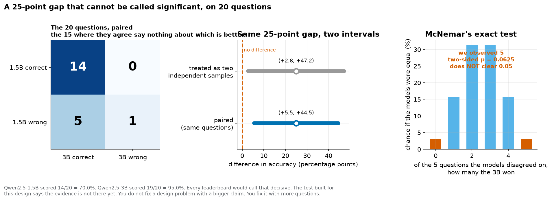— Figure 3:**A 25-point gap that cannot be called significant, on twenty questions.** The left panel is the contingency table: the fifteen questions on the main diagonal, fourteen both-right and one both-wrong, say nothing about which model is better. The middle panel is the same 25-point gap with two different intervals around it, from Formulas 13.9 and 13.10; both exclude the dashed line at zero. The right panel is the distribution McNemar’s test actually uses: if the two models were equally good, the five disagreements would split like five coin tosses, and the bars show how likely each split would be. The observed split was five to nothing, and doubling the end probability gives $p = 0.0625$ . Drawn by `lab/fig_extra.py` from `lab/out/we7_paired.json`.

Try it 13.3: Run McNemar’s test yourself

The numbers in this box are made up for practice. No model produced them.

Two models answer the same 30 questions. Both are right on 18, both wrong on 4, only model B is right on 7, and only model A is right on 1.

Check the table adds up.
How many discordant pairs are there, and what are model A’s and model B’s accuracies?
Compute the two-sided exact p-value.
State the conclusion in a sentence a non-statistician would understand.

You will need these “choose” values: $\binom{8}{0} = 1$ and $\binom{8}{1} = 8$ . And $\left(\tfrac{1}{2}\right)^{8} = 1 \div 256 = 0.00390625$ .

13.9 How many questions would it actually take?¶

Intuition¶

Something in section 13.8 should have bothered you, and if it did not, here it is.

McNemar’s test on five disagreements returned 0.0625. Now ask: what is the smallest p-value that five disagreements could ever produce?

The most extreme outcome possible is a clean sweep: all five going the same way. That is what happened. There is no more lopsided result available. So 0.0625 is not an unlucky value, it is the floor. With five disagreements, the smallest two-sided p-value that exists is 0.0625.

Which means this: the study could not have produced a significant result no matter how the two models performed. Even if the 3B had been perfect and the 1.5B hopeless on those five, the answer would still have been 0.0625, and 0.0625 is still above 0.05.

That is not a fact about these two models. It is a fact about a twenty-question benchmark with fifteen agreements in it. The design was incapable of answering the question before either model was loaded.

This is worth more than it might look. It means you can check whether a comparison is worth running before you run it. Count the disagreements you expect, work out the floor, and if the floor is above 0.05, you already know the answer will be “cannot tell” and you can go and build a bigger bank instead of burning an afternoon.

The threshold turns out to be six. Six disagreements give a floor of 0.03125, which is below 0.05. Five give 0.0625, which is not. So a paired comparison of two models needs at least six questions on which they disagree before it can possibly reach significance, and that is before you ask anything about how lopsided the split has to be.

How many questions does that mean? It depends entirely on how often the models disagree. Here, five disagreements came out of twenty questions, a disagreement rate of one in four. Two models that are close in ability disagree rarely, which is exactly when you most need the test to work.

The literature has a number for this. Miller (arXiv:2411.00640) recommends that a model evaluation contain at least 1,000 questions to signal reliably. Twenty is one fiftieth of that. The recommendation lands differently when you have hit the wall yourself in section 13.8 than when somebody tells you at the start.

The mathematics¶

Formula 13.12: The smallest p-value a design can produce

1. In words. Take the number of items the two systems disagreed on. The most lopsided result possible is all of them going the same way. The chance of that, doubled for a two-sided test, is the smallest p-value that design can ever return. If that number is above your threshold, no outcome can be called significant.

2. The formula.

p_{\min} = 2 \left(\frac{1}{2}\right)^{m}

3. The symbols.

Symbol	How to say it out loud	What it means
$p_{\min}$	“p min”	the answer: the smallest two-sided p-value this design could ever give
the subscript “min”	“min”, short for minimum	it marks this as the smallest possible value, not the one you observed
$=$	“equals”	the two sides are the same number
2	“two”	doubling, for a two-sided test
the 2 and the bracket written side by side	“times”	two things written next to each other with no sign between them means multiply them. See the toolkit on multiplication
$\left(\frac{1}{2}\right)^{m}$	“a half to the power m”	a half multiplied by itself $m$ times. See the toolkit on exponents
$m$	“em”	the number of discordant pairs, $b + c$ . A plain $m$ , not the $m_j$ of Formula 13.4, which counted how often one option was chosen

4. Out loud. “The smallest possible p-value is two times a half raised to the power of the number of disagreements.”

5. Worked, for every small number of disagreements. Build the ladder one rung at a time. Each rung is the one above it divided by 2.

$m = 1$ : $\left(\tfrac{1}{2}\right)^{1} = 0.5$ , and $2 \times 0.5 = 1.0$

$m = 2$ : $\left(\tfrac{1}{2}\right)^{2} = 0.25$ , and $2 \times 0.25 = 0.5$

$m = 3$ : $\left(\tfrac{1}{2}\right)^{3} = 0.125$ , and $2 \times 0.125 = 0.25$

$m = 4$ : $\left(\tfrac{1}{2}\right)^{4} = 0.0625$ , and $2 \times 0.0625 = 0.125$

$m = 5$ : $\left(\tfrac{1}{2}\right)^{5} = 0.03125$ , and $2 \times 0.03125 = \mathbf{0.0625}$

$m = 6$ : $\left(\tfrac{1}{2}\right)^{6} = 0.015625$ , and $2 \times 0.015625 = \mathbf{0.03125}$

The crossing happens between five and six. At $m = 5$ the floor is 0.0625, above the 0.05 line. At $m = 6$ it is 0.03125, below it.

6. Check it. $p_{\min}$ must fall between 0 and 1, and at $m = 1$ it is exactly 1, which is correct and is the sanity check for the whole formula: a single disagreement can never be evidence of anything, and a p-value of 1 says precisely that.

Each rung must be exactly half the one above it. $1.0, 0.5, 0.25, 0.125, 0.0625, 0.03125$ . ✅ If yours does not halve each time, check your powers of two. See the toolkit on powers of two.

Python¶

# For each possible number of disagreements, the smallest two-sided p the design can ever give.
print("disagreements   smallest possible two-sided p   can it ever reach 0.05?")
for possible_discordant_pairs in range(1, 9):
    smallest_possible_p = 2 * (0.5 ** possible_discordant_pairs)
    print("     ", str(possible_discordant_pairs).rjust(2), "        ",
          str(round(smallest_possible_p, 6)).rjust(10), "                  ",
          smallest_possible_p < 0.05)

Output:

disagreements   smallest possible two-sided p   can it ever reach 0.05?
       1                 1.0                    False
       2                 0.5                    False
       3                0.25                    False
       4               0.125                    False
       5              0.0625                    False
       6             0.03125                    True
       7            0.015625                    True
       8            0.007812                    True

range(1, 9) gives the numbers 1 through 8; it starts at the first number and stops before the second. 0.5 ** possible_discordant_pairs raises a half to that power. The comparison smallest_possible_p < 0.05 produces True or False, and printing it puts the verdict straight into the table.

The False on the fifth row is the whole section. Five disagreements cannot produce a significant result. The lab’s comparison had five disagreements. Its verdict was decided by the size of the bank, before either model was loaded onto the graphics card.

Try it 13.4: Is the comparison worth running?

The pilot in this box is made up for practice. No such pilot was run.

You are planning a comparison of two models on a bank you are about to build. From a pilot on ten questions, the two models disagreed on 2 of them, so you estimate a disagreement rate of about one question in five.

How many questions would you need for about 6 disagreements?
At that size, could the comparison reach $p < 0.05$ ?
Would 6 disagreements be enough for you to be comfortable? Give a reason either way.

13.10 The failure taxonomy, at last¶

Intuition¶

You have met model failure many times by now, in a different costume almost every week, and this book has not once stopped to sort those failures into kinds. That was deliberate. Naming the kinds in Week 1 would have handed you vocabulary for things you had not yet seen. Naming them here gives you names for things you have already watched happen, argued about in section, and measured yourself.

Here are six kinds, each one anchored to a measurement in this book.

1. Tokenizer failure. The model never sees the thing you typed. It sees pieces. The string '1234567' becomes seven separate tokens, one per digit, which is the mechanical reason these models are bad at arithmetic. Chapter 2.

2. Harness failure. The tooling around the model quietly changes the question. Asking Ollama for the continuation of The capital of France is without setting raw mode makes the model answer a chat turn instead, and the “next token” came back as 'The' at 99.9993%. That looks like a model with no uncertainty at all, and it is an artefact of the harness. Chapter 1 is where local running and hosted running are set beside each other. The 99.9993% itself is recorded in _research/00-lab-verified-findings.md, section 1.

3. Numerical failure. The arithmetic that stores the model loses something. Quantizing to four bits with one scale for the whole tensor gave a mean weight error of 46.6% of the weights’ own standard deviation, because a single large outlier set the scale. With one scale per block of 32 weights, the same four bits gave 7.2%. Chapter 7.

4. Retrieval failure. The model is given the wrong evidence and answers from it faithfully. Fixed-window chunking of the CSUB compendium put the correct section at rank 1 on essentially no question, because every requirement list reads alike and a window starting mid-section does not know which section it is in. Chapter 10.

5. Fabrication. The model produces fluent, confident text that is false. Asked to continue The capital of France is, the 0.5B model wrote “Paris. It was founded in 789 AD”, and Paris is roughly a thousand years older than that. Nothing in the machinery checks facts. Probability is about which text is likely, never about which text is true. Chapter 10 is where retrieval is offered as a partial repair. The sentence itself is printed in the Python reference appendix, from lab/out/appendix_python_reference_checks.json.

6. Measurement failure. Your instrument is bent and the number it gives you is about the instrument. The naive scorer made the model answer A on 16 of 20 questions and reported 25.0%. This chapter.

Now count. Of those six, exactly one is the model being bad at its own job. That is number 5, fabrication. The other five are failures of something you built around the model: how you cut the text, how you called the tool, how you stored the numbers, how you chose the passages, how you marked the answers.

That is the most useful thing in the taxonomy and it is the reason it lands in this chapter rather than in Week 1. Most of what looks like a model failing is a procedure failing. You have to be able to tell the two apart, and you can only tell them apart by measuring your measurement.

The mathematics¶

One small formula, and it is the hinge into Chapter 14.

Formula 13.13: An accuracy restricted to one kind of item

1. In words. Instead of the share right across all the questions, take the share right across only the questions of one particular kind. Count how many of that kind the model got right, divide by how many of that kind there were.

2. The formula.

\hat{p}_K = \frac{x_K}{n_K}

3. The symbols.

Symbol	How to say it out loud	What it means
$\hat{p}_K$	“p hat sub K”	the answer: the accuracy on items of kind $K$ alone
the hat	“hat”	measured, not known for certain
$K$	“kay”, capital	which kind of item. Here, a topic: centre, spread, probability, and so on
$=$	“equals”	the two sides are the same number
$x_K$	“x sub K”	how many items of kind $K$ the model got right
the fraction bar	“divided by”	divide the top by the bottom
$n_K$	“n sub K”	how many items of kind $K$ there were in total

4. Out loud. “The accuracy on a kind is the number of that kind got right, divided by the number of that kind asked.”

5. Worked, on the real run. In lab/out/we6_eval.json, the naive run’s results are broken down by topic. Two of the topics:

On design questions, the model got 2 of 2 right.

\hat{p}_{\text{design}} = \frac{2}{2} = 2 \div 2 = 1.0, \qquad 1.0 \times 100 = 100.0\%

On spread questions, it got 0 of 3 right.

\hat{p}_{\text{spread}} = \frac{0}{3} = 0 \div 3 = 0.0, \qquad 0.0 \times 100 = 0.0\%

The overall score was 25.0%. Neither of those two topic scores is anywhere near 25%.

6. Check it. $\hat{p}_K$ must land between 0 and 1. And the check that matters most: a subgroup accuracy computed from a handful of items carries an enormous interval. Two questions is not a measurement of anything. The 100% on design questions rests on two questions, and Chapter 12 is where you learned what two questions buys you.

The point of Formula 13.13 here is not to report those two numbers as findings. It is that an overall score can hide a topic at 100% and a topic at 0% inside it, and Chapter 14 is about what happens when the kinds are groups of people rather than topics in statistics.

Python¶

# Six kinds of failure this book has measured, each with the chapter that met it and the
# number that proves it. Every value here is quoted from _research/00-lab-verified-findings.md.
failure_kinds = [
    ["tokenizer", 2, "'1234567' becomes 7 separate tokens"],
    ["harness", 1, "Ollama without raw mode returned 'The' at 99.9993 percent"],
    ["numerical", 7, "4-bit per-tensor quantization: 46.6 percent mean weight error"],
    ["retrieval", 10, "fixed-window chunking put the right section at rank 1 on essentially no question"],
    ["fabrication", 10, "the model wrote that Paris was founded in 789 AD"],
    ["measurement", 13, "the naive scorer made the model answer A on 16 of 20 questions"],
]

print("kind          first met   what was measured")
for one_kind in failure_kinds:
    name_of_kind = one_kind[0]
    chapter_number = one_kind[1]
    the_evidence = one_kind[2]
    print(name_of_kind.ljust(14), ("Ch " + str(chapter_number)).ljust(11), the_evidence)

print("kinds of failure named:", len(failure_kinds))

# Only one of the six is a failure of the model on its own terms.
failures_of_our_procedure = 0
for one_kind in failure_kinds:
    if one_kind[0] in ["tokenizer", "harness", "numerical", "retrieval", "measurement"]:
        failures_of_our_procedure = failures_of_our_procedure + 1
print("kinds that are failures of the procedure, not of the model:", failures_of_our_procedure, "of", len(failure_kinds))

Output:

kind          first met   what was measured
tokenizer      Ch 2        '1234567' becomes 7 separate tokens
harness        Ch 1        Ollama without raw mode returned 'The' at 99.9993 percent
numerical      Ch 7        4-bit per-tensor quantization: 46.6 percent mean weight error
retrieval      Ch 10       fixed-window chunking put the right section at rank 1 on essentially no question
fabrication    Ch 10       the model wrote that Paris was founded in 789 AD
measurement    Ch 13       the naive scorer made the model answer A on 16 of 20 questions
kinds of failure named: 6
kinds that are failures of the procedure, not of the model: 5 of 6

A list of lists is a list whose items are themselves lists. failure_kinds[0] is the whole first row, and failure_kinds[0][1] is the 2 in it. Inside the loop, one_kind[0] is the name, one_kind[1] the chapter, one_kind[2] the evidence. The in on the second-to-last loop asks “is this value one of the items in that list”, and gives back True or False.

Five of six. That ratio is not a law of nature and this book is not claiming it is; it is a count of the failures this particular course chose to teach. What it does capture is the working habit: when something goes wrong, your first suspect is the thing you built, not the model.

Try it 13.5: Name the failure

The four situations in this box are made up for practice. None of them was measured.

For each of these, name which of the six kinds it is, and say what measurement you would run to confirm your diagnosis.

A model is asked “what is 847 plus 296” and answers 1133 instead of 1143.
A model summarising a Kern County water report cites a figure that does not appear anywhere in the report.
A model scored 88% on a benchmark last month, and 61% this month, on the same questions and the same weights. The evaluation code was updated in between.
A model shrunk to run on a 4 GB laptop starts producing broken words and repeated phrases.

Common mistakes¶

Reporting a score without the procedure. “The model scored 35%” is half a sentence. The whole sentence is “the model scored 35% under length-normalised option-text scoring, on this twenty-question bank.” If you cannot say the second half, you do not have a result yet.
Treating a score near chance as a measurement of the model. It might be. Check the instrument first. A score that lands on the guessing rate is a prompt to inspect the scoring procedure, not a finding about knowledge.
Comparing a score against the wrong chance level. The 25% line belongs to a procedure that asks each question once. The rotation procedure asks four times and needs three hits, and its chance level is 5.1%, from Worked example 13.2. Judged against 25% the rotation score of 15.0% looks worse than guessing. Judged against its own 5.1% it is three times chance. Work out the chance level of the procedure you actually used.
Assuming debiasing always lowers a score. It lowered the 0.5B by 10 points and the 1.5B by 10 points, and moved the 3B by nothing at all. The gap is a symptom that shows up when a model is weak. There is no fixed correction to apply.
Fixing a bias and not re-checking. Scoring the option text raised the score to 35% and left an answer spread of A 7, B 11, C 2, D 0 against a key of A 2, B 8, C 8, D 2. The old bias went away and a new one arrived. Always re-print the spread after a fix.
Using the unpaired formula on paired data. If both models answered the same questions, the unpaired standard error is the wrong tool. It is not catastrophic here, 1.14 times wider, and it is free to do it properly.
Adding the two pieces outside the square root. In Formula 13.9 both fractions sit under one root. Taking two roots and adding them gives 0.1512 instead of 0.1135, which is wrong by a third.
Running McNemar on all the items. The concordant pairs take no part in the test. Only the disagreements do. Using $n = 20$ instead of $m = 5$ turns the test into something else.
Forgetting to double for a two-sided test. $\left(\tfrac{1}{2}\right)^5 = 0.03125$ is the one-sided answer and it clears 0.05. The two-sided answer is 0.0625 and it does not. Unless you decided in advance that only one model could possibly be better, the test is two-sided.
Reading $p = 0.0625$ as “the models are the same”. It says twenty questions cannot tell them apart. The 3B may well be better; you have not measured it yet. Absence of evidence is not evidence of absence.
Reading $p = 0.0625$ as “the probability the models are equal is 6.25%”. A p-value is computed assuming the models are equal, so it cannot also be a verdict on whether they are.
Confusing percentages with percentage points. Going from 70% to 95% is a rise of 25 percentage points. It is a rise of about 36 per cent of the original value, because $25 \div 70 = 0.357$ , and then $0.357 \times 100 = 35.7$ , which rounds to 36. These are different numbers and reporting the wrong one inflates or deflates your result. See the toolkit.
Quoting a metric without reading its definition. The consistency count in this chapter means “the four rotations agreed on the verdict”, which is not quite the same as “gave the same answer four times”. The rule applies to this book’s numbers too.

What to remember¶

An evaluation score is a property of the scoring procedure at least as much as of the model, and the same model on the same twenty questions scored 25.0%, 35.0% and 15.0% under three defensible rules. A score sitting on the chance level is a reason to inspect the instrument, and inspecting it here showed a model answering A on 16 of 20 questions while the key rewarded A twice. Position bias is a symptom of a weak model rather than a fixed tax: the debiasing gap was 10 points at 0.5B, 10 points at 1.5B and 0 points at 3B. When two models answer the same questions, compare them question by question, because the items they agree on carry no information about which is better. And a 25-point gap can fail to be significant: five disagreements, all one way, give McNemar’s exact $p = 0.0625$ , which does not clear 0.05, so the answer is more questions rather than a bigger claim.

Practice problems¶

Some of these problems reuse the chapter’s own measured numbers, and those name the model or the section they came from. Every other number in this section is made up for practice. The invented ones are built to be checkable by hand, and none of them is a measurement of anything.

The answers appendix works the chapter’s McNemar calculation in full, and the answers to the odd-numbered problems below are being added there in problem-number order. Bring the even-numbered ones to section.

Warm-up: can you do the arithmetic?¶

1. A model gets 9 of 20 questions right. Write that as a decimal and as a percentage.

2. A benchmark has questions with five options each and exactly one correct answer. What is the chance level, as a decimal and as a percentage?

3. A 40-question bank has four options per question. How many questions would a random guesser be expected to get right?

4. On a 20-question bank, a scoring procedure chose option D twelve times. Compute the over-choice ratio for D, using Formula 13.4.

5. Turn each of these into the other form: 0.45 into a percentage; 62% into a decimal; 17 out of 25 into a percentage.

6. Compute $\left(\tfrac{1}{2}\right)^{6}$ by halving six times, showing each halving.

7. A model scored 60% naive and 45% debiased on the same bank. What is the debiasing gap in percentage points?

8. A contingency table reads: both right 22, both wrong 6, only model B right 9, only model A right 3. Check that it adds up, and say how many questions there were and how many disagreements.

Practice: can you apply it?¶

9. A 25-question bank has four options. A procedure chose A eleven times, B six, C five, D three. Compute the over-choice ratio for every option, and check that the four ratios average to 1.

10. The same procedure scored 36%. The answer key spread is A 5, B 7, C 8, D 5. Write three sentences saying what you suspect about the procedure and what you would measure next.

11. A four-option question has its correct answer in position 2, which is option C. Using Formula 13.6, work out where the correct answer sits after each of the four cyclic rotations, and check that all four positions are visited exactly once.

12. Two options are scored. The first is 3 tokens with log-probabilities -0.7, -1.4 and -0.6. The second is 6 tokens with log-probabilities -0.9, -0.8, -1.0, -0.7, -1.1 and -0.8. Which option wins on totals, and which wins after length normalisation? Show every step.

13. Model A scores 0.55 and model B scores 0.80, each on 40 questions. Compute the unpaired standard error using Formula 13.9, and give the 95% interval for the difference in percentage points.

14. Two models on 25 shared questions: both right 15, both wrong 3, only B right 6, only A right 1. Build the paired difference, its standard deviation and its standard error, and give the 95% interval. Show each step the way Formula 13.10 does.

15. For the table in problem 14, run McNemar’s exact test. You will need $\binom{7}{0} = 1$ , $\binom{7}{1} = 7$ and $\left(\tfrac{1}{2}\right)^{7} = 0.0078125$ .

16. Using Formula 13.12, find the smallest number of disagreements that could ever produce a two-sided p-value below 0.01. Show the ladder.

17. A colleague reports: “Our model beat theirs, 78% to 71%, on our 100-question internal benchmark.” Write five questions you would ask before believing it. For each one, say what a bad answer would look like.

18. A model scored 3 of 3 on questions about one topic and 1 of 12 on another, for an overall score of 4 of 15. Compute all three accuracies using Formula 13.13, then write one sentence saying why you would not report the 100% without a qualifier.

Stretch: can you reason with it?¶

19. The naive procedure in this chapter chose option C zero times out of twenty, and C was correct on eight questions. Work out the highest score that procedure could possibly have reached on this bank, and explain in your own words why every reported benchmark score has a ceiling set by its procedure.

20. Section 13.5 argues that a model always picking position A scores exactly one of four on every question under rotation. Write out that argument as carefully as you can, then work out what a model that always picks position A and always picks position B on alternate askings would score. State any assumption you had to make.

21. The 1.5B model has a debiasing gap of 10 points but a letter spread of C 7, B 7, D 2, A 4, which does not lean towards any one position. Propose two different explanations for a non-zero debiasing gap that is not driven by a simple position preference, and for each one describe a measurement that would tell the two explanations apart.

22. Suppose you re-ran the whole two-model comparison on a fresh bank of 20 questions drawn from the same source, and got a contingency table of both right 13, both wrong 2, only 3B right 4, only 1.5B right 1. Compute McNemar’s exact p. Then discuss: your two studies now disagree about the direction of one question. What would you do next, and what would you refuse to do?

23. McNemar’s test and the paired Wald interval gave opposite verdicts on the same data in this chapter. Explain, in a paragraph a classmate could follow, why they disagree and why this book believes McNemar. Then name one situation in which you would trust the Wald interval more.

24. Design a study that could actually detect a 10 percentage point difference between two models. State the disagreement rate you are assuming and where that assumption comes from, the number of disagreements you need, the bank size that implies, and what you would do if the real disagreement rate turned out to be half what you assumed. Miller (arXiv:2411.00640) is a reasonable starting point, and you should say how your number compares with the 1,000 it recommends.

25. Worked example 13.2 found that a guesser scores about 5.1% under a majority-of-four rule on four-option questions. Now change the rule to “majority of three rotations, meaning at least two hits out of three” and work out the chance level for that, showing every multiplication. You will need $\binom{3}{2} = 3$ . Then say which of the two rules you would rather report a score under, and why “the one with the lower chance level” is not a good enough reason on its own.

What comes next¶

Chapter 14 takes Formula 13.13 and changes what the kinds are. Instead of topics in statistics, the kinds become groups of people, and the question becomes whether a model that scores well on average scores well for everybody. Then it puts a price on the compute that produced the score and asks who is paying it.

The habit this chapter built is the one you carry into that. Before you argue about a number, find out how it was made.