Quantization: what you lose, what it buys
MATH 3219, Chapter 7: rounding a model down, and why the same arithmetic is an energy argument and an access argument
Chapter 7. Quantization: what you lose, what it buys
What you need before this chapter
This chapter needs sixteen pieces of notation and one idea from Chapter 6. Every one of them has a section in the Math Toolkit that starts from nothing. If a symbol on this page stops you, follow its link, read that section, and come back. That is what the links are for.
| You will meet | Toolkit section |
|---|---|
| A letter standing for a number, such as for “how many bits” | Section 1, a letter standing for a number |
| Subscripts, such as for “weight number ” | Section 2, subscripts |
| Multiplication, written as and also by writing two symbols side by side | Section 3, multiplication |
| The fraction bar, which means divide | Section 4, the fraction bar |
| Exponents, such as 23 | Section 5, exponents |
| Absolute value, the two upright bars in | Section 15, absolute value and magnitude |
| Rounding to the nearest whole number | Section 16, rounding and significant figures |
Scientific notation, such as 109, which the code writes as 1e9 | Section 17, scientific notation |
| Powers of two, and what a bit is | Section 18, powers of two |
| The sign, used once, in Section 7.4 | Section 10, sigma notation |
| The square root sign, , used twice, in Section 7.4 | Section 9, square roots |
| The standard deviation, which you will work out by hand in Section 7.4 | Section 10, the standard deviation |
| Percentages, used everywhere | Section 11, percentages |
| Percentage points, which are not the same as percent | Section 11, percentage points |
| Reading a bar chart | Section 13, reading a graph |
| The sign, “is less than or equal to”, used in Section 7.8 | Section 19, inequality signs |
From Chapter 6 you need one sentence: a number format with fewer bits can represent fewer different values, so more numbers have to be rounded. If that sentence makes sense to you, you are ready. If it does not, read Chapter 6 first, because this chapter is what happens when you push that idea as far as it will go.
You do not need calculus. You do not need to have programmed. Every piece of arithmetic on this page can be done on a phone calculator, and most of it is division.
The setup code
Run this once, at the top of your session, before anything else on this page. Every line has a comment saying what it is for. Nothing here computes anything yet; it tells Python which tools you are about to use.
# Cell 1. Run this once at the top of the session.

import os                                       # lets Python read and change settings on your computer
os.environ.setdefault("HF_HUB_DISABLE_SYMLINKS_WARNING", "1")   # hides a Windows-only warning about model files
os.environ["HF_HOME"] = r"C:\math3219\models"  # where the models are kept; MUST come before the transformers line
import json                                     # reads the .json files the lab scripts wrote
import torch                                    # the arithmetic library the language models are built on
import matplotlib.pyplot as pyplot              # draws every chart in this book
from transformers import AutoModelForCausalLM   # loads a model that predicts the next token

okabe_ito_vermillion = "#D55E00"   # the colour this book uses for the method that fails
okabe_ito_green = "#009E73"        # the colour this book uses for the method that works
okabe_ito_grey = "#999999"         # the colour this book uses for reference lines

print("torch version:", torch.__version__)
print("setup finished")
Output on the course machine:
torch version: 2.6.0+cu124
setup finished
Two of those lines deserve a word. import torch brings in the whole arithmetic library under
its own name, so later you write torch.round(...). from transformers import AutoModelForCausalLM reaches into a library and pulls out one named piece, so later you write
AutoModelForCausalLM.from_pretrained(...) with no transformers. in front of it. The three
colour names are the book’s palette, chosen so that readers with colour vision deficiency can
still tell the bars apart.
A laptop in Bakersfield, in August
Here is the situation this chapter exists to change.
A student opens a laptop in a study room on the CSU Bakersfield campus. She wants the model
that works. In this course that is Qwen2.5-3B-Instruct, and on the twenty-question bank in
Chapter 13 it answers 19 of them correctly, a score of 95.0%. Twenty questions is a small test,
so that 95.0% comes with a wide margin of error, and Section 7.8 prints it rather than leaving it
out. She types the two lines of Python that load it. The machine thinks for a moment and then
refuses. The message is about memory.
The model needs 6.17 gigabytes of graphics memory to hold its numbers. Her graphics card has 4 gigabytes. The gap is 2.17 gigabytes, and it is not a gap in her preparation, her question, or her ability. It is a gap in her hardware, and it decided what she was allowed to ask.
That is the whole problem, and it is not hypothetical. The three models in this course need 0.99, 3.09 and 6.17 gigabytes at half precision. A 4 gigabyte card, which is an ordinary card, fits the first two and not the third. The line falls between the model that scores 70.0% and the model that scores 95.0%, both on the same small test and both with the wide intervals that Section 7.8 reports.
Now the second half of the same situation. That graphics card, while it works, draws electrical power. On the machine this book was written on, the card drew a mean of 21.3 watts while the smallest model wrote, and 30.2 watts while the largest one did. Almost all of that power leaves the card as heat. In a Bakersfield August, that heat goes into a room that something else then has to cool. The course measures the card. It does not measure the air conditioner, and this chapter will keep saying so.
Two problems, then. Who can run it, and what it costs to run. The claim of this course is that they are not two problems. They are one problem, and the arithmetic in this chapter is where you can see them meet.
The arithmetic itself is rounding. That is all quantization is. You take every number inside the model and round it to one of a short list of allowed values, so that each one fits in fewer bits. Done carelessly, this destroys the model, and you will watch it happen in Section 7.4: an ordinary weight inside a real attention matrix becomes exactly zero, and 46.6% of the spread of the weights is thrown away. Done the way real quantizers do it, the same four bits give an error of 7.2% instead, and the file goes from 0.988 gigabytes to 0.278 gigabytes.
The difference between those two outcomes is one decision about which numbers share a ruler. That is the chapter.
Learning objectives
By the end of this chapter you will be able to:
Explain what quantization is in plain language, and work out how many different values a given number of bits can store.
Compute a quantization scale by hand, then quantize and dequantize a single weight, and say how large the rounding error is.
Diagnose why one scale for a whole matrix fails, using the ratio between the largest weight and a typical weight, and predict which weights get erased.
Compute the storage cost of blockwise quantization honestly, including the bits spent on the block scales, and convert that into the size of the file on disk.
Join a measured energy figure to a measured accuracy figure and a measured memory figure, state what the joint picture recommends, and state precisely what the measurement leaves out.
This lesson at a glance
Quantization is rounding. Every weight is snapped to the nearest mark on a ruler, and the number of marks is set by how many bits you are willing to spend.
The ruler’s length is set by the largest weight that shares it. In a real matrix the largest weight is about 45 times a typical one, so one ruler for the whole matrix wastes almost all of its marks and erases ordinary weights.
One ruler per 32 weights fixes it. At 4 bits the mean error falls from 46.6% of the spread of the weights to 7.2%, for 12.5% more storage. Real quantizers do exactly this.
The same arithmetic is an energy argument and an access argument. Smaller models cost less energy per token and fit on cheaper machines, and on this course’s measurements both point at the same model.
The vocabulary of this chapter
Every term below is used later on this page. Read the table once now. You do not need to memorise it; you need to have seen the words before they arrive in a sentence.
| Term | What it means, in one line |
|---|---|
| weight | One of the learned numbers inside a model. A 0.5B model has 494,032,768 of them. |
| tensor | A grid of numbers. A weight matrix with 896 rows and 896 columns is a tensor. |
| bit | One binary digit, 0 or 1. It is the smallest unit of storage. |
| byte | Eight bits. |
| precision | How finely a number format can tell nearby values apart. |
| FP32, FP16, INT8 | Three ways to store one number: 32 bits, 16 bits, and 8 bits as a whole number. Chapter 6 covers the first two. |
| quantization | Rounding every weight to one of a small set of allowed values, and storing which one. |
| level | One of the allowed values a quantized weight is permitted to take. |
| scale | The gap between two neighbouring levels. It is the one extra number you must store. |
| quantize | To turn a weight into a whole number: divide by the scale and round. |
| dequantize | To turn that whole number back into a weight: multiply by the scale. |
| rounding error | The gap between the original weight and the value that comes back. |
| outlier | A weight far larger in size than the typical weight in the same tensor. |
| clipping | Chopping a weight that is too big down to the end of the ruler instead of lengthening the ruler. This chapter never clips. |
| per-tensor quantization | One scale shared by every weight in a tensor. The naive method. |
| block | A short run of consecutive weights, 32 of them in this book. |
| blockwise quantization | One scale per block, so an outlier can only spoil its 31 neighbours. |
| mean | The ordinary average. Add the numbers up, then divide by how many there are. |
| median | The middle value of a list once the list is sorted. Half the list is below it and half above. |
| variance | The average of the squared distances from the mean. Square root it and you have the standard deviation. |
| standard deviation | One number saying how spread out a set of numbers is. Written . |
| relative error | Mean rounding error divided by the standard deviation of the weights. |
| standard error | How much a measured score would move if you ran the same test on a fresh set of questions. Chapter 12 builds it. |
| GGUF | The single-file format llama.cpp and Ollama use to ship a quantized model. |
| K-quant | The family of blockwise schemes inside GGUF, with names like Q4_K_M. |
| watt (W) | A rate of energy use: one joule every second. |
| joule (J) | A unit of energy. One watt for one second. |
| watt-hour (Wh) | One watt kept running for an hour, which is 3,600 joules. |
| board power | What the whole graphics card draws, chip and memory and regulators together. |
| idle power | What the card draws with nothing running. It was 13.834 W on the lab machine. |
| energy per token | The electrical energy spent producing one token of output, in joules. |
| VRAM | Graphics memory. The model’s weights have to fit in it to run on the card. |
| lower bound | A number you are confident the truth is at least as large as. |
7.1 Rounding to a short list
Intuition
Think about the price of petrol. The sign on Rosedale Highway gives the price to a tenth of a cent, because petrol is sold in a way that makes tenths of a cent worth writing down. Now think about the price of a coffee. Nobody prices a coffee at two dollars, thirty-four and seventeen hundredths of a cent. The list of prices a shop actually uses is short, and every real price is snapped onto that short list.
Shortening a list is the whole idea. A shorter list of allowed values means each value needs less room to write down, because there are fewer of them to tell apart. If a shop only ever charges one, two, three or four dollars, you need two bits to record a price, because two bits can name four things. If it uses a hundred prices you need more.
Inside a language model the numbers are not prices, they are weights, the learned numbers that do the arithmetic. There are 494,032,768 of them in the smallest model in this course. Each one is normally stored in 16 bits, which is why the file is 0.988 gigabytes. The question this chapter asks is: what if you stored each one in 4 bits instead?
Four bits cannot hold an arbitrary decimal. Four bits can name sixteen things. So the model would have to pick sixteen allowed values, and round every weight to whichever one is nearest. Some weights would land exactly on an allowed value. Most would not, and would be nudged.
The nudging is what you pay. The bits you save are what you get. The whole of quantization is about making that trade well, and you will find that the trade is far more sensitive to which sixteen values you pick than to the fact that there are only sixteen.
Before any of that, you need to be able to answer one question: given bits, how many values can you name, and how many of them sit on each side of zero? That is Section 7.1’s formula, and it is the smallest formula in the chapter.
The mathematics
The weights in a model come in both signs. Some are positive, some are negative, and they sit roughly symmetrically around zero. So the levels should sit symmetrically around zero too: zero itself in the middle, some levels above it, the same number below.
Spend one bit on the sign, positive or negative. That leaves bits to say how big the number is. Those bits can name different sizes, and one of those has to be zero, because zero is a size a weight is allowed to have. So the number of non-zero steps available on each side of zero is .
That is the first formula of the chapter, and it gets the full six-part treatment every formula in this book gets.
Formula 1 of 12: how many whole steps fit on each side of zero
In words. One bit is spent saying whether the weight is positive or negative. The bits left over say how big it is. Work out how many different sizes those remaining bits can name, then take one away, because one of the sizes has to be zero itself.
The formula.
The symbols.
| Symbol | How to say it out loud | What it means |
|---|---|---|
| “steps” | the answer: how many non-zero levels sit on each side of zero | |
| “equals” | the thing on the left and the thing on the right are the same number | |
| 2 | “two” | the number two. It is two because a bit has two possible values, 0 and 1. |
| “bee” | how many bits you are spending on one stored weight | |
| “bee minus one” | one fewer than , because one bit was spent on the sign | |
| “two to the bee minus one” | 2 multiplied by itself times. See the toolkit on exponents. | |
| the raised position of | “to the power of” | a small raised number means “multiply the big number by itself this many times” |
| “minus” | subtract | |
| 1 | “one” | the number one |
Out loud. “The number of steps is two raised to one less than the number of bits, minus one.”
Worked, step by step, at 4 bits.
Step 1, work out . You have bits, so .
Step 2, raise 2 to that power. 23 means . The sign is the multiply sign. The toolkit covers it, and the three other ways this book writes the same instruction, in Section 3. Do it one multiplication at a time.
So .
Step 3, subtract 1. .
So 4 bits give 7 whole steps on each side of zero. The allowed level numbers run . Count them: 15 of them, plus one unused pattern, which is the sixteenth thing 4 bits can name.
Worked again, at 8 bits.
Step 1, .
Step 2, . Step by step: ; ; ; ; ; . So .
Step 3, .
So 8 bits give 127 steps each side.
Check it. The answer has to be a whole number, and it has to get bigger when gets bigger, because more bits can name more things. Going 2, 3, 4, 6, 8 bits should give 1, 3, 7, 31, 127, and each of those is one less than a power of two. If you get a number that is not one less than a power of two, you subtracted the 1 before raising to the power instead of after.
Python
Now open a real model and look at one real weight matrix, so the rest of the chapter has something concrete to work on. This cell downloads the model the first time you run it, which takes a minute or two on campus wifi, and then loads it from your own disk every time after that.
The matrix chosen is the query projection in the first attention layer. There is nothing special about it; it is the first weight matrix you meet if you open the model and walk in. Chapter 3 showed you where the parameters live, and this is one of the places they live.
# Cell 2. Open the model and take out one real weight matrix.

model_name = "Qwen/Qwen2.5-0.5B-Instruct"                # which model to fetch from the hub
language_model = AutoModelForCausalLM.from_pretrained(model_name, dtype=torch.float32).eval()   # download it once, then load it
weight_matrix = language_model.model.layers[0].self_attn.q_proj.weight.data.clone()   # one real matrix, copied so we cannot damage the model

print("shape of the matrix    :", tuple(weight_matrix.shape))
print("how many weights       :", weight_matrix.numel())
print("most negative weight   : %+.7f" % float(weight_matrix.min()))
print("most positive weight   : %+.7f" % float(weight_matrix.max()))
print("largest size, sign off : %.7f" % float(weight_matrix.abs().max()))
print("middle size (median)   : %.8f" % float(weight_matrix.abs().median()))
print("standard deviation     : %.6f" % float(weight_matrix.std()))
Output:
shape of the matrix    : (896, 896)
how many weights       : 802816
most negative weight   : -1.2265625
most positive weight   : +1.1718750
largest size, sign off : 1.2265625
middle size (median)   : 0.02697754
standard deviation     : 0.066741
Read that output line by line, because the rest of the chapter is an argument about those seven numbers.
shape is , meaning 896 rows and 896 columns. Multiply them and you get
, which is the second line. This one matrix holds 802,816 learned
numbers, and it is one matrix out of hundreds in a model that has 494,032,768 numbers in total.
The third and fourth lines are the extremes. The most negative weight is -1.2265625 and the
most positive is +1.1718750. The fifth line, largest size, sign off, throws away the minus
signs and asks which weight is largest in size. That is 1.2265625, the negative one. Size
with the sign thrown away is called absolute value, and it is written with two upright bars:
. The toolkit covers it in
Section 15.
The sixth line is the one to hold on to. The median size is 0.02697754. Median means middle: line all 802,816 sizes up from smallest to largest and take the one in the middle. Half the weights in this matrix are smaller in size than 0.02697754, and half are larger. So 0.02697754 is what a typical weight in this matrix looks like.
Put the fifth and sixth lines next to each other. The largest weight is 1.2265625. The typical weight is 0.02697754. One of them is about 45 times the other. That single comparison is what makes Section 7.4 go wrong, and everything from here to there is building the machinery to see why.
The last line, the standard deviation, is 0.066741. It is one number describing how spread out the whole set of weights is. It will be the denominator in Section 7.4 when you need to say how bad an error is in a way that does not depend on the units.
.numel() means “number of elements”. .abs() throws away minus signs. .max(), .median()
and .std() do what they say. dtype=torch.float32 asks for the weights at full 32-bit
precision, so that any rounding you see later is rounding you did, not rounding that was
already in the file.
7.2 The scale: how far apart the marks are
Intuition
Picture a ruler with no numbers printed on it, only tick marks, and you get to decide two things before you use it: how many tick marks there are, and how long the ruler is.
The number of tick marks is set by your bit budget. Section 7.1 settled that: with bits you get marks on each side of zero. At 4 bits that is 7 marks up and 7 marks down. That number is fixed and you cannot argue with it.
The length of the ruler is the interesting decision, and it is not free either. The ruler has to reach the largest weight it is responsible for. If a weight in the matrix has size 1.2265625 and your ruler only reaches 0.5, that weight cannot be written down at all. It would have to be chopped off at the end of the ruler, which is a much worse error than rounding. So the ruler has to be at least as long as the largest weight that will use it.
Once you have fixed the number of marks and the length, the gap between neighbouring marks follows automatically. Spread 7 marks evenly over a length of 1.2265625 and each gap is . The sign says divide the number on its left by the number on its right. It is the same instruction as the fraction bar you will meet in Formula 2, written on one line instead of two. The toolkit treats the two together in Section 4. That gap is called the scale, and it is the single most important number in this entire chapter.
Here is why it matters so much. Every weight gets snapped to the nearest mark. If the gap between marks is large, the snap can move a weight a long way. If the gap is small, the snap barely moves it. So the scale controls the damage. And the scale is set by the largest weight sharing the ruler, not by the typical one.
Read that last sentence twice. Whatever sets the scale sets it for everything the scale covers. A quantizer does not choose a nice round scale; the biggest weight in the group hands it one. If one weight in a group of 802,816 is enormous, then all 802,816 of them get a ruler sized for that one weight, and the other 802,815 are rounded on a ruler far too long for them.
That is the failure this chapter is built around. You are two formulas away from seeing it happen to a real number.
The mathematics
One question has to be settled before the formula makes sense: why must the ruler reach all the way to the largest weight? Why not make it shorter, so the marks are closer together, and accept that a few very large weights fall off the end?
You could. The technique is called clipping, and it means replacing any weight past the end of the ruler with the value at the end. It is a real method and Practice problem 24 asks you to work one out. The reason this chapter does not start there is that clipping trades one kind of damage for another, and the damage it introduces is not rounding. A rounded weight moves to a neighbouring mark. A clipped weight moves as far as you like, and it is the biggest weights in the model that get moved. Large weights are not noise; a weight that is 45 times a typical one is doing something the training put there on purpose.
So the scheme in this chapter never clips. The ruler always reaches the largest weight in the group it serves, and the only decision left is how many marks to put on it. That decision is the bit budget, and the gap between marks follows from the two together.
Formula 2 of 12: the quantization scale
In words. Find the largest weight in the group, ignoring its minus sign if it has one. Divide that by the number of whole steps available on each side of zero. The answer is how far apart the allowed values have to be.
The formula.
The symbols.
| Symbol | How to say it out loud | What it means |
|---|---|---|
| “ess” | the answer: the scale, the gap between two neighbouring allowed values | |
| “equals” | the two sides are the same number | |
| “w sub i” | weight number in the group. The small underneath is a counter: is the first weight, the second. See the toolkit on subscripts. | |
| “the absolute value of w sub i” | the size of that weight with its minus sign thrown away. and . | |
| the two upright bars | “absolute value” | the throw-away-the-sign instruction. They have nothing to do with division. |
| “the maximum over i” | look at every weight in the group, one at a time, and keep the biggest answer | |
| “two to the bee minus one, minus one” | the number of whole steps on each side of zero, straight from Formula 1 | |
| “bee” | how many bits you are spending on one stored weight | |
| the fraction bar | “divided by” | divide the number above the bar by the number below it. See the toolkit on the fraction bar. |
Out loud. “The scale is the largest weight size in the group, divided by the number of whole steps that fit on each side of zero.”
Worked, step by step, at 4 bits, on the real matrix.
This is a real measurement, not a made-up number. The largest weight size in
layers[0].self_attn.q_proj.weight is 1.2265625, printed by Cell 2 above.
Step 1, get the number of steps from Formula 1. At : , then , then .
Step 2, divide the largest weight size by that.
If you want to check the division on a calculator: , which is 1.2265625 to seven decimal places.
So at 4 bits, with one ruler for the whole matrix, neighbouring allowed values are 0.17522321 apart.
Worked again, at 8 bits.
Step 1, , then , then steps.
Step 2, .
Check it. Three checks, and they catch almost every slip.
First, the scale is always positive, because the top of the fraction is an absolute value and the bottom is a count.
Second, the scale gets bigger as gets smaller. Fewer bits means fewer marks spread over the same length, so the gaps are wider. Compare the two answers: 8 bits gave 0.00965797 and 4 bits gave 0.17522321, which is about 18 times wider. If your scale went down when you took bits away, you have the fraction upside down.
Third, and this is the direct one, divide the largest weight by your scale and you must land exactly on the top step. , which is the 7 from Step 1. If you get something else, you used the wrong .
Python
The code below does Formula 2 five times, once for each bit width the lab measured. It is a
for loop: the indented lines run once for every value in the list after in. Nothing is
hidden inside a function, so you can read the arithmetic straight down the page.
# Cell 3. The scale, for one ruler covering the whole matrix.

largest_weight_size = float(weight_matrix.abs().max())   # the biggest size in the matrix

print("bits   whole steps each side        scale")
for bit_width in (8, 6, 4, 3, 2):                        # run once for each of these five
    whole_steps = 2 ** (bit_width - 1) - 1               # Formula 1
    per_tensor_scale = largest_weight_size / whole_steps # Formula 2
    print("%4d %22d %12.8f" % (bit_width, whole_steps, per_tensor_scale))
Output:
bits   whole steps each side        scale
   8                    127   0.00965797
   6                     31   0.03956653
   4                      7   0.17522321
   3                      3   0.40885417
   2                      1   1.22656250
Five lines, and each one is the two formulas you have met. Read down the middle column first: 127, 31, 7, 3, 1. Every one of those is one less than a power of two, which is the check from Formula 1.
Now read down the right column: 0.00965797, 0.03956653, 0.17522321, 0.40885417, 1.22656250. The gaps get wider every row. That is the second check from Formula 2, and here it is happening five times in a row.
Look hard at the bottom row. At 2 bits there is exactly one step on each side of zero, and the scale is 1.22656250, which is the largest weight itself. A 2-bit quantizer with one ruler for this matrix can store only three values: -1.2265625, 0, and +1.2265625. Every one of the 802,816 weights has to become one of those three numbers. You can already guess what happens to a weight of size 0.027.
In Python, ** means “raised to the power of”, so 2 ** (bit_width - 1) is . The
brackets matter: Python would work out 2 ** bit_width - 1 as and then subtract one,
which is a different and wrong number. The %12.8f inside the print line means “print this
number in a column 12 characters wide with 8 digits after the decimal point”, which is what keeps
the columns lined up. float(...) turns the single number torch hands back into an ordinary
Python number, so the arithmetic on the next line is ordinary arithmetic.
One more thing about the loop. The variable whole_steps is computed fresh on every pass. It is
127 on the first pass, 31 on the second, and so on. Nothing carries over between passes except
largest_weight_size, which was computed once, before the loop, because the matrix does not
change.
7.3 What happens to one weight
Intuition
You now have a ruler. Time to use it on something.
The action has two halves and they happen at different times. The first half happens once, when the model is shrunk: take a weight, work out which mark on the ruler it is nearest to, and write down the number of that mark. Not the weight. The mark number, which is a small whole number like -3 or 0 or +5. That whole number is what gets stored in the file, and it is small enough to fit in four bits.
The second half happens every single time the model runs: take the stored mark number, multiply it by the scale, and you have a weight again. Not the original weight. The value of the mark it was snapped to.
Those two halves are called quantize and dequantize. Quantize is divide and round. Dequantize is multiply. They are opposites in the same way that “round to the nearest dollar” and “that is how many dollars” are opposites, which is to say they are not really opposites at all, because the rounding threw something away and no amount of multiplying brings it back.
The thing thrown away is the rounding error: the gap between the weight you had and the weight you get back. It is the price of the whole exercise.
Here is the part that surprises people. The rounding error on one weight does not depend on how big that weight is. It depends on how close the weight happened to land to a mark. A weight sitting almost exactly on a mark comes back almost perfectly. A weight sitting halfway between two marks comes back off by half a scale. The error can never be worse than half a scale, because the nearest mark is never further away than that.
So the size of the scale caps the damage. And the scale, from Section 7.2, is set by the largest weight in the group. You are one formula away from the collision.
The mathematics
Formula 3 of 12: quantize, then dequantize
In words. Divide the weight by the gap between marks, and round to the nearest whole number. That whole number says which mark it landed on, and that is what gets stored. To read the weight back later, multiply the stored whole number by the gap between marks.
The formula.
The symbols.
| Symbol | How to say it out loud | What it means |
|---|---|---|
| “q sub i” | the whole number stored in place of weight . It lies between and . | |
| “equals” | the two sides are the same number | |
| “round” | round to the nearest whole number. 2.4 becomes 2, 2.6 becomes 3, -1.9 becomes -2. See the toolkit on rounding. | |
| the round brackets after | “of” | they say what is being rounded: everything inside them |
| “w sub i” | the original weight, before anything was done to it | |
| “ess” | the scale, from Formula 2 | |
| the fraction bar | “divided by” | divide the top by the bottom |
| the comma | no sound | it separates two formulas that are carried out one after the other |
| “w hat sub i” | the dequantized weight: the number the model actually uses after shrinking | |
| the hat, | “hat” | a small mark meaning “this stands in for the real thing, it is not the real thing” |
| the gap between and | “times” | two symbols written side by side are multiplied together |
Out loud. “The stored number is the weight divided by the scale, rounded to the nearest whole number. The weight you get back is that stored number multiplied by the scale.”
Worked, step by step, at 8 bits, on the real typical weight.
The weight is . This is the median-magnitude weight of the real matrix, so half the matrix is smaller than this in size. It is an utterly ordinary weight.
Step 1, write down the scale for 8 bits, from Section 7.2: . That scale is itself a rounded number, printed to eight decimal places, so every answer below carries that rounding. The computer keeps more digits of the scale, so its answers differ from these by one unit in the last digit printed. The book shows both rather than hiding the difference, and the paragraph under Cell 4 says exactly where the two part company.
Step 2, divide the weight by the scale.
Step 3, round to the nearest whole number. The value -2.793293 sits between -3 and -2. How far is it from each? From -3 it is 0.206707 away; from -2 it is 0.793293 away. It is nearer to -3, so .
Step 4, multiply back by the scale to dequantize.
Step 5, work out the rounding error. Take the sizes and subtract.
So at 8 bits the weight moved by about two thousandths. It survived.
Worked again, at 4 bits, on the same weight.
Step 1, the 4-bit scale from Section 7.2: .
Step 2, divide. .
Step 3, round. The value -0.153961 sits between -1 and 0. From -1 it is 0.846039 away; from 0 it is 0.153961 away. It is nearer to 0, so .
Step 4, multiply back. .
Step 5, the rounding error is the whole weight: 0.02697754.
The weight did not shrink. It was deleted. The model will use zero where a real learned number used to be.
Check it. Two checks.
The stored number must be a whole number inside the allowed range. At 4 bits the range is -7 to +7, and 0 is inside it.
The rounding error can never be larger than half the scale. At 4 bits, half the scale is , and the error 0.02697754 is smaller than that, so the arithmetic is consistent. If your error comes out larger than half the scale, you rounded the wrong way.
Python
The next cell does Formula 3 on the real typical weight at every bit width. It first has to find that weight, which takes two lines worth explaining.
weight_matrix.flatten() takes the 896-by-896 grid and lays it out as one long row of 802,816
numbers, in reading order: first row left to right, then second row, and so on. torch.argsort
then sorts those numbers by size and hands back the positions, smallest first. Taking the
position halfway along that sorted list gives the weight whose size is in the middle, which is
the median weight.
# Cell 4. What per-tensor quantization does to one ordinary weight.

all_weights_in_a_row = weight_matrix.flatten()                       # 802,816 numbers in one row
order_by_size = torch.argsort(all_weights_in_a_row.abs())            # positions, smallest size first
middle_position = int(order_by_size[all_weights_in_a_row.numel() // 2])   # the position halfway along
typical_weight = float(all_weights_in_a_row[middle_position])        # the weight at that position

print("the typical weight is %+.8f" % typical_weight)
print()
print("bits        scale   weight/scale   stored   comes back as        error")
for bit_width in (8, 6, 4, 3, 2):
    whole_steps = 2 ** (bit_width - 1) - 1                     # Formula 1
    per_tensor_scale = largest_weight_size / whole_steps       # Formula 2
    weight_over_scale = typical_weight / per_tensor_scale      # the division in Formula 3
    stored_whole_number = int(round(weight_over_scale))        # the rounding in Formula 3
    comes_back_as = stored_whole_number * per_tensor_scale     # dequantize
    rounding_error = abs(comes_back_as - typical_weight)       # how far off we are
    print("%4d %12.8f %14.6f %8d %+15.8f %12.8f"
          % (bit_width, per_tensor_scale, weight_over_scale,
             stored_whole_number, comes_back_as, rounding_error))
Output:
the typical weight is -0.02697754

bits        scale   weight/scale   stored   comes back as        error
   8   0.00965797      -2.793292       -3     -0.02897392   0.00199638
   6   0.03956653      -0.681827       -1     -0.03956653   0.01258899
   4   0.17522321      -0.153961        0     +0.00000000   0.02697754
   3   0.40885417      -0.065983        0     +0.00000000   0.02697754
   2   1.22656250      -0.021994        0     +0.00000000   0.02697754
This is the single most important output in the chapter. Take it row by row.
The 8-bit row. The weight divided by the scale is -2.793292, which rounds to -3, and -3 times the scale is -0.02897392. The error is 0.00199638. The weight survived with a small nudge. Compare that to the hand arithmetic four paragraphs above, which gave -2.793293 and then -0.02897391. Both differ from the computer’s answer in the last digit printed, and for one reason: by hand you divided by the scale rounded to eight decimal places, while the computer used 0.009657972440944882. Neither answer is wrong. The rounding is carried through, and it moves the last digit. It does not move the rounded whole number , which is -3 either way, so the conclusion is unchanged.
The 6-bit row. The weight divided by the scale is -0.681827, which rounds to -1, so the weight comes back as -0.03956653. Notice what happened: the weight got bigger, from 0.02698 to 0.03957 in size. Rounding does not always shrink a number. It moves it to the nearest mark, in whichever direction that is.
The 4-bit row. The weight divided by the scale is -0.153961. The nearest whole number to -0.153961 is zero. So the stored number is 0, the weight comes back as 0, and the error is the entire weight, 0.02697754.
The 3-bit and 2-bit rows. The same thing, more so. -0.065983 and -0.021994 both round to zero.
Say what that means plainly. At 4 bits with one scale for the whole matrix, the median weight of a real attention matrix is erased. The median. Half the weights in the matrix are smaller in size than this one, and the nearest mark to every one of them is also zero. So somewhat more than half of this matrix becomes exactly zero, and the model is being asked to do arithmetic with the holes.
If you stopped reading here, you would conclude that 4-bit quantization destroys language models. Many people have concluded exactly that. It is wrong, and Section 7.5 shows why, but the conclusion is a reasonable one to draw from this table, and this book would rather show you the failure than skip to the fix.
7.4 Why one scale for the whole matrix fails
Intuition
Something has gone wrong, and it is worth being precise about what.
It is tempting to say “four bits is not enough”. That is not the problem. Four bits give you fifteen usable levels, and fifteen levels is plenty to describe a weight of size 0.027 if the levels are in the right place. The problem is that the levels are in the wrong place. They are at 0, , , , and so on up to . The sign ± is read “plus or minus”, and it is a way of writing two numbers at once: means the pair +0.175 and -0.175, one level above zero and its mirror image below. A weight of size 0.027 is nowhere near any of them except zero.
Why are they there? Because the ruler had to reach 1.2265625, the largest weight in the matrix. Stretch seven marks across that distance and the first mark lands at 0.175, which is already six and a half times the size of a typical weight.
Now look at the shape of the data. The largest weight is 1.2265625. The median weight is 0.02697754. Divide one by the other and you get about 45. A single weight in this matrix is 45 times the typical one. Weights like that are called outliers, and language models are full of them; it is not a defect in this matrix, it is how these models come out of training.
So the naive scheme spends its levels covering a range from 0.175 up to 1.227 where almost no weight lives, and has nothing left over for the range from 0 to 0.05 where most of them actually do live. It is a ruler designed entirely around its least representative measurement.
To argue about this properly you need a way to say how bad an error is. Saying “the mean error is 0.031” means nothing on its own, because you do not know whether 0.031 is large. Large compared to what? Compared to the spread of the weights themselves. If the weights are typically 0.067 apart in the sense that the standard deviation measures, then an error of 0.031 is about half the spread, and that is catastrophic. That comparison is the second formula of this section.
The mathematics
Formula 4 of 12: the outlier ratio
In words. Take the size of the largest weight in the group. Take the size of the middle weight in the group. Divide the first by the second. The answer tells you how many times bigger the worst case is than the typical case, and therefore how badly a single shared ruler will be stretched.
The formula.
The symbols.
| Symbol | How to say it out loud | What it means |
|---|---|---|
| “are” | the answer: the ratio. It has no units, because it is a size divided by a size. | |
| “equals” | the two sides are the same number | |
| “w sub i” | weight number in the group. See the toolkit on subscripts. | |
| the two upright bars in | “absolute value” | the throw-away-the-sign instruction, so . They have nothing to do with division. See the toolkit on absolute value. |
| “the maximum over i of the absolute value of w sub i” | the size of the biggest weight in the group, sign thrown away | |
| “the median over i of the absolute value of w sub i” | line every size up from smallest to largest and take the one in the middle | |
| “median” | the middle value of a sorted list. It is not the mean. | |
| the small under and | “over i” | it says to run the counter over every weight in the group before taking the answer |
| the fraction bar | “divided by” | divide the top by the bottom |
Out loud. “R is the size of the largest weight divided by the size of the middle weight.”
Worked, step by step, on the real matrix.
Both numbers were printed by Cell 2 and neither was invented.
Step 1, the largest size: 1.2265625.
Step 2, the median size: 0.0269775391.
Step 3, divide.
To check that division without a calculator, go the other way: , and . The true value 1.2265625 sits between those two, so the answer is between 45 and 46. It is 45.47.
Check it. is a size divided by a size, so it can never be negative. And it can never be less than 1, because the largest value in a list cannot be smaller than the middle value of that same list. If you get a number below 1, you have the fraction upside down. A value of exactly 1 would mean every weight in the group has the same size, which does not happen in a real model.
One borrowed formula first: the standard deviation
Formula 5 divides by the standard deviation of the weights, so you need to be able to work one out before Formula 5 will mean anything. The standard deviation is not a quantization idea and it is not invented here. It belongs to the Math Toolkit, which builds it from nothing. It is restated here in full, because you are about to compute one by hand, twice.
One warning about the letters before you start. The toolkit writes the standard deviation as . This chapter has already given to the quantization scale, and two different meanings for one letter on one page would be cruel. So on this page the standard deviation is written , never , and always means the scale.
In words. The standard deviation is a typical distance from the average. Work out how far each number is from the average of all of them. Square those distances, so that a number below the average and a number above it both count as being away from it. Average the squares. Then take a square root, which undoes the squaring and brings the answer back into the same units as the numbers you started with.
The formula.
The symbols.
| Symbol | How to say it out loud | What it means |
|---|---|---|
| “the standard deviation of w” | the answer, in the same units as the weights | |
| “equals” | the two sides are the same number | |
| “the square root of” | the tick-with-a-roof sign. The square root of a number is the number that gives it back when multiplied by itself: because . Everything under the long bar goes inside. See the toolkit on square roots. | |
| “en” | how many numbers are in the list | |
| “en minus one” | one fewer than the count. You divide by this rather than by when the list is a sample of something larger, which a set of weights is. Chapter 12 says why. | |
| “minus” | subtract | |
| “the sum from i equals 1 to en” | add up whatever follows, once for each number in the list. See the toolkit on sigma notation. | |
| “sigma” | the capital Greek letter S. It is an instruction to add things up, nothing more. See the toolkit on Greek letters. | |
| “eye” | a counter. means the first number, the second. | |
| the fraction and the sum written side by side | “times” | two things written next to each other with no sign between them are multiplied. See the toolkit on multiplication. |
| “w sub i” | number in the list | |
| “w bar” | the average of all the numbers. The bar on top is what marks it as an average. | |
| “w sub i minus w bar” | how far this number sits from the average. It is negative when the number is below the average. | |
| the round brackets | “bracket” | they say to do the subtraction first, before squaring |
| “all squared” | multiply the bracket by itself. Squaring always gives a positive answer. | |
| the fraction bar | “divided by” | divide the sum above it by the below it |
Out loud. “The standard deviation is the square root of, one over en minus one, times the sum of each number minus the average, all squared.”
Worked, step by step, on three numbers. Made up for practice. The three numbers are 2, 4 and 9.
Step 1, find the average. Add them, then divide by how many there are.
So .
Step 2, subtract the average from each number.
Step 3, square each of those.
Step 4, add the squares.
Step 5, divide by , which is .
Step 6, take the square root. Your calculator has a key.
So .
Check it. Three checks. The differences in Step 2 must add to zero: , and they do; if they do not, the average is wrong. Every square in Step 3 must be positive; a negative one is a sign error. And the answer must be smaller than the full range of the numbers, which is here, and 3.605551 is. To check the square root itself, multiply it by itself: , which is 13 to five decimal places.
Formula 5 of 12: relative error, the honest way to report damage
In words. Work out how far off each weight is, ignoring whether it is off upwards or downwards, and average those over all the weights. Then divide that average by how spread out the weights were in the first place. Reporting the error as a share of the spread makes “how bad is 4-bit?” a question with an answer that does not depend on what the numbers are measured in.
The formula.
The symbols.
| Symbol | How to say it out loud | What it means |
|---|---|---|
| “relative error” | the answer. It comes out as a plain decimal, and you turn it into a percentage by multiplying by 100. See the toolkit on percentages. | |
| “equals” | the two sides are the same number | |
| “en” | how many weights are in the group. For this matrix, . | |
| “the sum from i equals 1 to en” | add up whatever follows, once for each weight, starting at weight 1 and finishing at weight . See the toolkit on sigma notation. | |
| “sigma” | the capital Greek letter S. It is an instruction to add things up, nothing more. | |
| “w hat sub i” | the weight you get back after quantizing, from Formula 3 | |
| “w sub i” | the original weight | |
| “w hat sub i minus w sub i” | the error on that one weight. It can be positive or negative. | |
| the two upright bars | “absolute value” | throw away the minus sign, so that an error upwards and an error downwards do not cancel each other out |
| “one over en” | multiplying by one over is the same as dividing by , which is how you take an average | |
| “the standard deviation of w” | one number saying how spread out the original weights are. A bigger value means they are further apart. It is the borrowed formula set out above, and also in the toolkit. | |
| the big fraction bar | “divided by” | divide the average error above it by the spread below it |
Out loud. “The relative error is the average size of the rounding errors, divided by the standard deviation of the weights themselves.”
Worked, step by step, on four weights. Made up for practice.
Real matrices have 802,816 weights and nobody is adding those up by hand. These four are invented so the arithmetic is short. The last of the four is the real typical weight; the other three are chosen to keep the numbers tidy.
The four weights are 0.10, -0.06, 0.03 and -0.02697754, quantized at 4 bits with the whole-matrix scale .
Step 1, quantize and dequantize each one with Formula 3.
| rounds to | error | |||
|---|---|---|---|---|
| 0.10000000 | 0.570701 | 1 | 0.17522321 | 0.07522321 |
| -0.06000000 | -0.342420 | 0 | 0 | 0.06000000 |
| 0.03000000 | 0.171210 | 0 | 0 | 0.03000000 |
| -0.02697754 | -0.153961 | 0 | 0 | 0.02697754 |
Step 2, add the four errors, one addition at a time.
Step 3, divide by to get the average error.
Step 4, work out the standard deviation of the four original weights, using the borrowed formula from a few paragraphs back. First find their average.
Step 5, subtract that average from each weight and square the result. Squaring means multiplying a number by itself, and it makes every answer positive.
Step 6, add those four squares.
Step 7, divide by , then take the square root. You divide by one fewer than the count because these four weights are a sample of a much larger set, which is the reason given in the borrowed formula above. The square root undoes the squaring, so the answer comes back in the same units as the weights. It is the key on your calculator, and the toolkit starts from zero on it.
Step 8, divide the average error by the standard deviation.
Step 9, turn that into a percentage by multiplying by 100. A percentage is a share written as a number out of a hundred, so multiplying a decimal by 100 is the whole of the conversion. The toolkit on percentages starts from zero on this.
, which is to one decimal place.
What the real matrix gives. Those four weights were made up. Across all 802,816 real weights, the measured mean error at 4 bits per-tensor is 0.031098 and the measured standard deviation is 0.066741. Divide:
That is the number quoted in the course description, and it lives in lab/out/we3b_quant.json.
Check it. Relative error can never be negative, because the top is built from absolute values and the bottom is a standard deviation, and neither can go below zero. It should also fall as you spend more bits. If your relative error goes up when you add bits, you used the wrong scale somewhere.
Python
The next cell puts Formula 4 and Formula 5 together on the real matrix. It is the first cell that
touches all 802,816 weights at once, and the trick that makes that fast is that torch applies an
operation to an entire tensor in one go. weight_matrix / per_tensor_scale divides every one of
the 802,816 numbers by the scale, all at once.
# Cell 5. The outlier ratio, and what it costs across the whole matrix.

middle_weight_size = float(weight_matrix.abs().median())        # the typical size
outlier_ratio = largest_weight_size / middle_weight_size        # Formula 4
spread_of_the_weights = float(weight_matrix.std())              # the sd in Formula 5

print("largest weight size  : %.7f" % largest_weight_size)
print("middle weight size   : %.10f" % middle_weight_size)
print("the ratio of the two : %.2f" % outlier_ratio)
print()
print("bits   mean error   as a share of the spread")
for bit_width in (8, 6, 4, 3, 2):
    whole_steps = 2 ** (bit_width - 1) - 1                      # Formula 1
    per_tensor_scale = largest_weight_size / whole_steps        # Formula 2
    per_tensor_stored = torch.clamp(torch.round(weight_matrix / per_tensor_scale),
                                    -whole_steps - 1, whole_steps)   # quantize, all at once
    per_tensor_back = per_tensor_stored * per_tensor_scale      # dequantize, all at once
    per_tensor_error = float((weight_matrix - per_tensor_back).abs().mean())   # top of Formula 5
    per_tensor_share = per_tensor_error / spread_of_the_weights # bottom of Formula 5
    print("%4d %12.6f %22.1f%%" % (bit_width, per_tensor_error, per_tensor_share * 100))
Output:
largest weight size  : 1.2265625
middle weight size   : 0.0269775391
the ratio of the two : 45.47

bits   mean error   as a share of the spread
   8     0.002413                    3.6%
   6     0.009800                   14.7%
   4     0.031098                   46.6%
   3     0.039294                   58.9%
   2     0.041820                   62.7%
The top three lines are Formula 4 on real data: the largest weight is about 45 times the middle one. The five rows underneath are Formula 5 at five bit widths.
At 8 bits the error is 3.6% of the spread of the weights, which is small enough to be unremarkable. At 6 bits it is 14.7%. At 4 bits it is 46.6%, meaning the average weight has been moved by almost half the spread of the whole distribution. At 2 bits it is 62.7%, and at that point the “model” is mostly zeros.
torch.round is the rounding step from Formula 3, applied to every weight at once.
torch.clamp(x, low, high) forces every value to stay inside a range, which matters because a
weight exactly at the top of the ruler could otherwise round to one step past the last level.
The range is to , which is why the code says
-whole_steps - 1, whole_steps.
.abs().mean() is the top of Formula 5, doing the sigma and the divide-by- in one move:
.abs() throws away the signs, .mean() adds them all up and divides by how many there are.
One caution on reading this table. These errors are about the weights, not about the answers the model gives. A weight error of 46.6% is alarming, and it is fair to expect a model in that state to be badly damaged, but this chapter has not measured its accuracy. That measurement is Lab 1, and this course does not let you claim a result it has not run. What this table establishes is narrower and still decisive: the naive scheme throws away a great deal, and the next section throws away far less for almost the same storage.
7.5 The fix: one ruler for every 32 weights
Intuition
Go back to the ruler. The problem was never the number of marks. The problem was that one ruler had to stretch all the way to the largest weight in 802,816 of them.
So stop using one ruler.
Chop the long row of weights into short runs of 32 in a row, and give each run its own ruler, sized by the largest weight in that run alone. A run of 32 is called a block. Now an outlier can only stretch the ruler belonging to the 31 weights sitting next to it. Everywhere else in the matrix, the ruler is sized by an ordinary local maximum, and the marks land where the weights actually are.
An everyday version. Suppose you are weighing things and your only scale reads up to 200 kilograms, in 15 steps, so the smallest thing it can distinguish is about 13 kilograms. That is fine for weighing people and useless for weighing letters. Nobody solves this by buying a scale with more steps. They use a kitchen scale for the letters and a bathroom scale for the people. Blockwise quantization is that: local rulers for local jobs.
The cost is bookkeeping. Every block now has its own scale, and every scale is a number you have to store. Section 7.6 counts exactly how much that costs, and the answer is 12.5% more storage at 4 bits. Hold that thought.
This is not a clever idea invented for a textbook. It is what real quantizers do. When you
download a model in GGUF format, the format llama.cpp and Ollama use, and the file name has
Q4_K_M in it, the K refers to K-quants, a family of blockwise schemes. Those schemes use
small blocks with their own scales, for this exact reason. The arithmetic you are about to do by
hand is a simplified version of what is running inside every quantized model anyone has on their
laptop.
The mathematics
Formula 6 of 12: the blockwise scale
In words. Split the weights into short runs. For each run on its own, find the largest weight in it, ignoring minus signs, and divide by the number of steps. That run gets its own gap between marks. Then quantize and dequantize every weight in the run using its own run’s gap.
The formula.
The symbols.
| Symbol | How to say it out loud | What it means |
|---|---|---|
| “kay” | which block you are talking about: block 1, block 2, block 3, and so on | |
| “ess bracket kay” | the scale belonging to block , and to no other block | |
| “equals” | the two sides are the same number | |
| the raised bracketed | “bracket kay” | a label saying which block. It is not an exponent. does not mean cubed. |
| “capital bee” | how many weights share one scale. in this book. | |
| “the maximum over i in block kay” | look only at the weights inside block , and keep the biggest size | |
| “in”, or “is an element of” | it says which weights you are allowed to look at | |
| “w sub i” | weight number , one of the weights inside block | |
| “absolute value of w sub i” | the size of the weight with its minus sign thrown away | |
| “bee” | how many bits you are spending on one stored weight | |
| “two to the bee minus one, minus one” | the number of whole steps each side of zero, exactly as in Formula 1 | |
| “q sub i” | the whole number stored for weight | |
| “round” | round to the nearest whole number | |
| “w hat sub i” | the weight that comes back after dequantizing | |
| the gap between and | “times” | two symbols written side by side with no sign between them are multiplied together. See the toolkit on multiplication. |
| the fraction bars | “divided by” | divide the top by the bottom |
| the commas | no sound | they separate three formulas carried out one after the other |
Out loud. “Each block gets its own scale, which is the largest weight size inside that block divided by the number of steps. Then every weight in the block is divided by that block’s scale and rounded, and multiplied back by that same scale to be read.”
Worked, step by step, on a block of four weights at 3 bits. Made up for practice.
Real blocks hold 32 weights. Four keeps the arithmetic short enough to do on a phone. The block is 0.08, -0.05, 0.02 and -0.03.
Step 1, find the largest size inside the block. The four sizes are 0.08, 0.05, 0.02 and 0.03. The largest is 0.08.
Step 2, get the number of steps from Formula 1. At : , then , then steps.
Step 3, divide to get this block’s scale.
That division does not come to an end. The 6 repeats forever, which the three dots say. So every written form of this scale is rounded, and below it is written 0.02666667, rounded to eight decimal places. The table in Step 4 keeps the repeating value underneath, so one of its entries differs in the last digit from what you get by multiplying the rounded 0.02666667 on a calculator. That is rounding travelling, and it never changes which mark a weight snaps to.
Step 4, quantize and dequantize each weight with that scale.
| rounds to | error | |||
|---|---|---|---|---|
| +0.08000 | +3.00000 | +3 | +0.08000000 | 0.00000000 |
| -0.05000 | -1.87500 | -2 | -0.05333333 | 0.00333333 |
| +0.02000 | +0.75000 | +1 | +0.02666667 | 0.00666667 |
| -0.03000 | -1.12500 | -1 | -0.02666667 | 0.00333333 |
Take the second row slowly. . That sits between -2 and -1. From -2 it is 0.125 away; from -1 it is 0.875 away. Nearer to -2, so . Then multiply back: , which the table prints as -0.05333333. On a calculator, with the rounded 0.02666667, you get -0.05333334 instead. That is the repeating digit showing up, and the error either way is .
Step 5, average the four errors.
Now do the same four weights with the whole-matrix scale, for contrast. At 3 bits the whole-matrix scale from Section 7.2 is .
| rounds to | error | |||
|---|---|---|---|---|
| +0.08000 | +0.19567 | 0 | 0 | 0.08000000 |
| -0.05000 | -0.12229 | 0 | 0 | 0.05000000 |
| +0.02000 | +0.04892 | 0 | 0 | 0.02000000 |
| -0.03000 | -0.07338 | 0 | 0 | 0.03000000 |
Every one of them rounds to zero. The average error is .
Compare the two averages: 0.00333333 against 0.04500000. The block version is times better, on the same weights, at the same 3 bits, with the same formula. The only thing that changed is which maximum you divided by.
Check it. Three checks.
Inside a block, the largest weight must come back almost exactly, because it sits on the top mark by construction. In the table above, 0.08 came back as exactly 0.08000000. Check that first, always.
A block scale can never be larger than the whole-matrix scale, because the largest weight in one block cannot be bigger than the largest weight in the whole matrix. So blockwise error can never be worse, on average, than per-tensor error. If yours is worse, you took the maximum over the wrong set of weights.
And the error on any single weight still cannot exceed half that weight’s own block scale. Half of 0.02666667 is 0.01333333, and the biggest error in the table is 0.00666667, which is under it.
Python
First, find out which block the typical weight lives in and what that block’s largest weight is. This is real, not made up: every weight in the matrix has a definite position, and position 587,210 is where the median weight sits.
# Cell 6. The block that the typical weight actually lives in.

block_size = 32
which_block = middle_position // block_size                  # // divides and throws away the remainder
first_position_in_block = which_block * block_size
last_position_in_block = first_position_in_block + block_size - 1
this_block = all_weights_in_a_row[first_position_in_block:last_position_in_block + 1]
block_largest_size = float(this_block.abs().max())           # the max in Formula 6

print("the typical weight sits at position :", middle_position)
print("so it belongs to block number       :", which_block)
print("that block covers positions         :", first_position_in_block,
      "to", last_position_in_block)
print("largest size inside that block      : %.11f" % block_largest_size)
print("largest size in the whole matrix    : %.7f" % largest_weight_size)
Output:
the typical weight sits at position : 587210
so it belongs to block number       : 18350
that block covers positions         : 587200 to 587231
largest size inside that block      : 0.07568359375
largest size in the whole matrix    : 1.2265625
There is the whole argument of the chapter in two numbers. The largest weight anywhere in the matrix is 1.2265625. The largest weight in the block of 32 that our typical weight actually lives in is 0.07568359375. Divide one by the other: . The local ruler is about sixteen times shorter, which means its marks are about sixteen times closer together, which means the rounding is about sixteen times finer, at the same 4 bits.
// is integer division: it divides and throws away the remainder, so
with a remainder, and // reports 18350. The slice
all_weights_in_a_row[587200:587232] takes the 32 numbers from position 587,200 up to but not
including position 587,232.
Now run Formula 6 on that block at every bit width.
# Cell 7. The same weight, quantized inside its own block of 32.

print("bits        scale   weight/scale   stored   comes back as        error")
for bit_width in (8, 6, 4, 3, 2):
    whole_steps = 2 ** (bit_width - 1) - 1                   # Formula 1
    block_scale = block_largest_size / whole_steps           # Formula 6, first part
    weight_over_scale = typical_weight / block_scale         # Formula 6, second part
    stored_whole_number = int(round(weight_over_scale))      # the rounding
    comes_back_as = stored_whole_number * block_scale        # Formula 6, third part
    rounding_error = abs(comes_back_as - typical_weight)
    print("%4d %12.8f %14.6f %8d %+15.8f %12.8f"
          % (bit_width, block_scale, weight_over_scale,
             stored_whole_number, comes_back_as, rounding_error))
Output:
bits        scale   weight/scale   stored   comes back as        error
   8   0.00059593     -45.269355      -45     -0.02681702   0.00016052
   6   0.00244141     -11.050000      -11     -0.02685547   0.00012207
   4   0.01081194      -2.495161       -2     -0.02162388   0.00535366
   3   0.02522786      -1.069355       -1     -0.02522786   0.00174967
   2   0.07568359      -0.356452        0     +0.00000000   0.02697754
Put this table next to the one in Section 7.3 and read the 4-bit row of each.
Per-tensor at 4 bits: the weight comes back as +0.00000000. Erased.
Blockwise at 4 bits: the weight comes back as -0.02162388. The sign is right, the size is roughly right, and the model has a real number to work with instead of a hole.
The 2-bit row still fails, and it should. Two bits give one step each side of zero, so the only values available are -0.0757, 0 and +0.0757, and our weight of size 0.027 is nearer to zero than to 0.0757. Blocks do not make two bits enough. Nothing makes two bits enough for this weight, and the honest thing is to say so.
Here is that measurement, both schemes side by side, all 802,816 weights.
# Cell 8. Per-tensor and blockwise, measured across the whole matrix.

print("bits   per-tensor error   share   blockwise error   share")
for bit_width in (8, 6, 4, 3, 2):
    whole_steps = 2 ** (bit_width - 1) - 1

    per_tensor_scale = largest_weight_size / whole_steps                 # one ruler for everything
    per_tensor_stored = torch.clamp(torch.round(weight_matrix / per_tensor_scale),
                                    -whole_steps - 1, whole_steps)
    per_tensor_back = per_tensor_stored * per_tensor_scale
    per_tensor_error = float((weight_matrix - per_tensor_back).abs().mean())

    weights_in_rows_of_32 = all_weights_in_a_row.view(-1, block_size)    # 25,088 rows of 32
    block_scales = weights_in_rows_of_32.abs().amax(dim=1, keepdim=True) / whole_steps
    block_stored = torch.clamp(torch.round(weights_in_rows_of_32 / block_scales),
                               -whole_steps - 1, whole_steps)
    block_back = block_stored * block_scales
    block_error = float((weights_in_rows_of_32 - block_back).abs().mean())

    print("%4d %18.6f %6.1f%% %17.6f %6.1f%%"
          % (bit_width, per_tensor_error,
             per_tensor_error / spread_of_the_weights * 100,
             block_error, block_error / spread_of_the_weights * 100))
Output:
bits   per-tensor error   share   blockwise error   share
   8           0.002413    3.6%          0.000266    0.4%
   6           0.009800   14.7%          0.001090    1.6%
   4           0.031098   46.6%          0.004831    7.2%
   3           0.039294   58.9%          0.011211   16.8%
   2           0.041820   62.7%          0.029854   44.7%
Read the 4-bit row across: 46.6% against 7.2%. Same matrix, same four bits, same rounding rule. The only difference is that the left-hand column used one ruler for 802,816 weights and the right-hand column used 25,088 rulers, one per block of 32.
.view(-1, block_size) re-lays the long row of 802,816 numbers as a grid with 32 columns.
The -1 tells torch to work out the number of rows itself, and it works out
exactly, with no remainder, which is why this code needs no
special handling for a leftover part-block. .amax(dim=1, keepdim=True) takes the largest value
along each row, which is the maximum over each block, which is the top of Formula 6.
Two honest notes on this table.
At 2 bits, blockwise still gives 44.7%, which is bad. Blocks help at every bit width, and they do not rescue every bit width. The gap between the columns is widest at 8 bits, where blockwise is about nine times better, and narrowest at 2 bits, where it is about 1.4 times better. When there are almost no levels left, no choice of ruler saves you.
And the whole table is about weights, not about answers. It says how much of the model’s arithmetic has been disturbed. Whether the model still answers questions is a separate measurement, and it belongs to Lab 1.
The same table is drawn below as a grouped bar chart. Each group along the bottom is one bit width. The two bars inside a group are the two schemes, and the height of a bar is the mean rounding error as a share of the spread, so a taller bar means worse rounding. If reading a bar chart is not something you do often, the toolkit starts from the axes in Section 13.
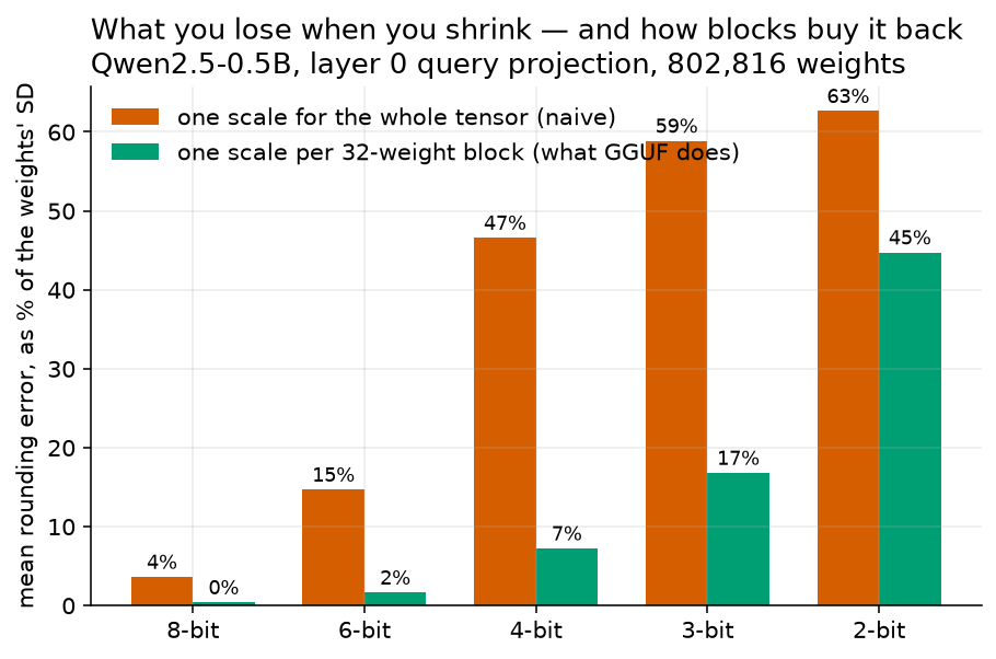
for Qwen2.5-0.5B, layer 0 query projection, 802,816 weights. The horizontal axis has five groups labelled 8-bit, 6-bit, 4-bit, 3-bit and 2-bit. The vertical axis is labelled “mean rounding error, as percent of the weights’ SD” and runs from 0 to a little above 60. Each group has two bars. The taller orange bar is one scale for the whole tensor and reads 4, 15, 47, 59 and 63 percent across the five groups. The shorter green bar is one scale per 32-weight block and reads 0, 2, 7, 17 and 45 percent. The orange bar is taller than the green bar in every group, and the difference is largest at 4-bit, where orange is 47 percent and green is 7 percent. :name: fig-ch07-quantization :width: 100%
The measurement of the whole chapter, in one chart. Mean rounding error as a share of the
weights’ standard deviation, at five bit widths, for one scale per tensor against one scale per
32-weight block. Both bars are labelled to the nearest whole percent; the table above gives the
same figures to one decimal place. Produced by lab/make_figures.py from
lab/out/we3b_quant.json.
Now put your hands on it. The simulation below shows one number line with the marks a chosen bit width allows, the true weight, and the value it snaps to. The two sliders are the two decisions this chapter is about: how many bits, and how long the ruler is. The weight on the line is the real -0.02697754.
Do one thing with it before you read on. Leave the bits at 4 and drag the scale maximum slowly from 0.05 up to 1.2266. Watch the “snapped value” readout. Long before you reach the top, the nearest mark stops being a neighbour of the weight and becomes zero, and it never comes back. Nothing about the weight changed. No bit was taken away. A distant outlier somewhere else in the same tensor stretched the ruler, and an ordinary weight was deleted.
Worked example 7.1: both schemes on the same eight weights
This is the whole of the first half of the chapter carried out by hand, on a set small enough to check on a phone. The eight weights are made up for practice, apart from the sixth, which is the real median weight -0.02697754. Real blocks hold 32 weights; eight keeps the arithmetic to one page.
The eight weights are
and they are quantized at bits both ways.
Part A, per-tensor. The scale comes from the whole matrix, so it is the computed in Section 7.2. Apply Formula 3 eight times.
| error | ||||
|---|---|---|---|---|
| +0.09000000 | +0.51363 | +1 | +0.17522321 | 0.08522321 |
| -0.07000000 | -0.39949 | 0 | 0 | 0.07000000 |
| +0.05000000 | +0.28535 | 0 | 0 | 0.05000000 |
| -0.04000000 | -0.22828 | 0 | 0 | 0.04000000 |
| +0.03000000 | +0.17121 | 0 | 0 | 0.03000000 |
| -0.02697754 | -0.15396 | 0 | 0 | 0.02697754 |
| +0.02000000 | +0.11414 | 0 | 0 | 0.02000000 |
| -0.01000000 | -0.05707 | 0 | 0 | 0.01000000 |
Seven of the eight rounded to zero. The one that did not, 0.09, came back as 0.17522321, which is nearly twice its true size.
Add the eight errors, one at a time.
Divide by 8 to get the mean error: .
Part B, blockwise. Treat the eight as one block. The largest size inside it is 0.09. From Formula 6, with 7 steps at 4 bits:
| error | ||||
|---|---|---|---|---|
| +0.09000000 | +7.00000 | +7 | +0.09000000 | 0.00000000 |
| -0.07000000 | -5.44444 | -5 | -0.06428571 | 0.00571429 |
| +0.05000000 | +3.88889 | +4 | +0.05142857 | 0.00142857 |
| -0.04000000 | -3.11111 | -3 | -0.03857143 | 0.00142857 |
| +0.03000000 | +2.33333 | +2 | +0.02571429 | 0.00428571 |
| -0.02697754 | -2.09825 | -2 | -0.02571429 | 0.00126325 |
| +0.02000000 | +1.55556 | +2 | +0.02571429 | 0.00571429 |
| -0.01000000 | -0.77778 | -1 | -0.01285714 | 0.00285714 |
Not one of them rounded to zero. Adding the eight errors gives 0.02269182, and .
Part C, compare. Divide one mean error by the other.
The blockwise result is about 14.6 times better on the same eight weights, at the same four bits, under the same rounding rule.
Part D, as a share of the spread. Formula 5 wants the standard deviation of the eight original weights. Their mean is
.
Now subtract that average from each of the eight weights and square the answer. Eight subtractions and eight multiplications, written out.
Add those eight, one addition at a time. Ten decimal places are kept here so the square root at the end lands on the same digits the computer gets.
Divide by . The answer is called the variance, which is the average of the squared distances, before the square root undoes the squaring.
Take the square root.
Per-tensor: , which is .
Blockwise: , which is .
Check it. The largest weight in the block, 0.09, came back exactly, which is the first check from Formula 6. The block scale 0.01285714 is smaller than the whole-matrix scale 0.17522321, which is the second check. And the pattern matches the real measurement: on the real 802,816 weights the same comparison at 4 bits gave 46.6% against 7.2%. The made-up numbers are not the same as the real ones, and they are not supposed to be. They show the mechanism; the table in Cell 8 is the measurement.
7.6 What the fix costs in storage
Intuition
Nothing is free, and blockwise quantization has a bill.
Each block of 32 weights now has its own scale, and that scale is a number the file has to carry. You cannot recover a weight without it: the stored value is a mark number like -2, and -2 is meaningless until you know how far apart the marks are.
So the file contains two kinds of thing. The mark numbers, four bits each, one per weight. And the scales, one per block. How many bits does a scale get? It gets 16, stored in half precision, which is the 16-bit format from Chapter 6, also written FP16. It gets that many because a rounded scale would corrupt every one of the 32 weights that depend on it. The one number you must not round is the number that tells you how much everything else was rounded.
Now count. A block of 32 weights at 4 bits each is bits. Add one 16-bit scale: bits per 32 weights. Share that out: bits per weight. So blockwise quantization at “4 bits” really costs four and a half bits per weight.
Four and a half against four is an overhead of 12.5%. That is the whole bill. For an eighth more storage, the mean error at 4 bits drops from 46.6% of the spread to 7.2% of it.
Then convert bits into something you can compare with a download. Eight bits make a byte, so 4.5 bits is bytes per weight. Multiply by the 494,032,768 parameters in the model and you have the size of the file. That arithmetic is the second formula of this section, and it is the one that answers the student in the study room.
The mathematics
Formula 7 of 12: bytes per weight, including the block scales
In words. Every block needs its own scale written down, and the scale takes room too. Count the bits spent on one weight, add that weight’s share of its block’s scale, and turn the total from bits into bytes.
The formula.
The symbols.
| Symbol | How to say it out loud | What it means |
|---|---|---|
| “bytes per weight” | the answer. It can be less than 1, which is the point of the exercise. | |
| “equals” | the two sides are the same number | |
| “bee” | bits spent on one stored weight, such as 4 | |
| “plus” | add | |
| “bee sub scale” | bits spent on one block scale. It is 16 in this book, because the scale is kept in half precision. | |
| “capital bee” | how many weights share that one scale. It is 32 in this book. | |
| the small fraction bar | “divided by” | dividing the scale’s bits by the number of weights sharing it gives each weight’s share of the bookkeeping |
| the big fraction bar | “divided by” | divide everything above it by the 8 below it |
| 8 | “eight” | there are 8 bits in a byte, so dividing by 8 turns bits into bytes |
Out loud. “Bytes per weight is the bits used for a weight, plus the bits used for a block scale shared out across the weights in that block, all divided by eight.”
Worked, step by step, for 4-bit weights with a 16-bit scale per 32 weights.
Step 1, work out the bookkeeping share. One scale, shared by 32 weights.
Step 2, add it to the bits spent on the weight itself.
Step 3, turn bits into bytes by dividing by 8.
Step 4, work out the overhead by comparing with the cost if you ignored the scales.
bytes per weight, and , so the bookkeeping costs 12.5% on top.
Check it. Multiply your answer by 8 and you must get back the total bits per weight: , which is Step 2. And when there are no block scales at all, the middle term is zero and the formula becomes . So 32-bit storage gives bytes per weight, which is what FP32 means, and 16-bit storage gives 2 bytes, which is what FP16 means. If those two do not come out right, the formula has been mistyped.
Formula 8 of 12: the size of the file
One convention has to be fixed before the formula, because the answer is quoted in gigabytes. Throughout this book GB means 109 bytes, which is a 1 followed by nine zeros, and which is how model files are usually quoted. That way of writing a large number is called scientific notation, and the toolkit covers it. Some tools use bytes instead and report a smaller-looking number for the same file. The bytes do not change; the divisor does. Say which convention you used.
In words. Multiply how many parameters the model has by how many bytes each one takes up. That is the size of the file you are about to download.
The formula.
The symbols.
| Symbol | How to say it out loud | What it means |
|---|---|---|
| “size in bytes” | the answer, in bytes | |
| “equals” | the two sides are the same number | |
| “en” | the parameter count. for Qwen2.5-0.5B-Instruct. | |
| “times” | multiply. See the toolkit on multiplication. | |
| “bytes per weight” | the answer from Formula 7 | |
| the round brackets | “bracket” | they group the quantity so you can see it counts as one number |
Out loud. “The size in bytes is the number of parameters multiplied by the number of bytes each parameter takes up.”
Worked, step by step, at FP16, which is what the model arrives as.
Step 1, write down the parameter count: .
Step 2, get the bytes per weight from Formula 7. FP16 means 16 bits with no block scales, so bytes.
Step 3, multiply.
Step 4, turn bytes into gigabytes by dividing by .
Worked again, at 4 bits with block scales.
Step 1, .
Step 2, bytes per weight from Formula 7: 0.5625.
Step 3, bytes.
If you want to do that multiplication in pieces: , and , and .
Step 4, GB.
Check it. Halving the bytes per weight has to halve the file size. Go down the list: FP32 is 1.976 GB, FP16 is 0.988 GB, INT8 is 0.494 GB, and each is half the one above. If yours do not halve, check whether you divided by 8 when turning bits into bytes. One more check on the size of the answer: half a billion numbers at four bytes each should be about 2 GB, and it is.
Python
Formula 7 and Formula 8 need two numbers each, and only one of them has to be measured: the parameter count. Everything else is a choice you make about the scheme. So the cell below starts by counting the parameters, then runs the same two formulas five times, once for each way of storing a weight.
The counting is the first three lines and it is worth reading slowly. number_of_parameters
starts at zero. The for loop then visits every tensor in the model in turn, asks it how many
numbers it holds, and adds that to the running total. When the loop finishes, the total is the
size of the model. There is no shortcut and there is not meant to be one; the loop is the
arithmetic, written out where you can see it.
Two lists follow. scheme_names holds the five labels, and scheme_bits holds the matching
bits-per-weight figure for each one, which is the top half of Formula 7. The fourth entry is
written as 4.0 + 16.0 / 32.0 rather than as 4.5, so that the two pieces of the formula stay
visible: four bits for the weight, and a sixteen-bit scale shared by thirty-two weights. Then a
second for loop walks the two lists together and does Formula 7 and Formula 8 on each row.
One piece of shorthand in the last line needs naming. 1e9 is how Python writes
, which is a 1 followed by nine zeros, or one billion. The e is not the number
and it is not an error; it is shorthand for “times ten to the power of”, and the digit after
it is the power. So size_in_bytes / 1e9 turns bytes into gigabytes under the convention fixed
above Formula 8. This way of writing large and small numbers is called scientific notation, and
the toolkit builds it from nothing.
# Cell 9. What the whole model costs on disk, under five schemes.

number_of_parameters = 0
for one_parameter_tensor in language_model.parameters():   # walk through every tensor in the model
    number_of_parameters = number_of_parameters + one_parameter_tensor.numel()

print("parameters in this model:", number_of_parameters)
print()
scheme_names = ["FP32", "FP16", "INT8", "4-bit + 16-bit scale per 32", "4-bit, scales ignored"]
scheme_bits = [32.0, 16.0, 8.0, 4.0 + 16.0 / 32.0, 4.0]     # the numerator of Formula 7
print("scheme                        bits/weight   bytes/weight   whole model")
for scheme_number in range(len(scheme_names)):              # 0, 1, 2, 3, 4
    bits_per_weight = scheme_bits[scheme_number]
    bytes_per_weight = bits_per_weight / 8.0                # Formula 7
    size_in_bytes = number_of_parameters * bytes_per_weight # Formula 8
    print("%-28s %12.4f %14.4f %9.3f GB"
          % (scheme_names[scheme_number], bits_per_weight, bytes_per_weight,
             size_in_bytes / 1e9))
Output:
parameters in this model: 494032768

scheme                        bits/weight   bytes/weight   whole model
FP32                              32.0000         4.0000     1.976 GB
FP16                              16.0000         2.0000     0.988 GB
INT8                               8.0000         1.0000     0.494 GB
4-bit + 16-bit scale per 32        4.5000         0.5625     0.278 GB
4-bit, scales ignored              4.0000         0.5000     0.247 GB
The first line is the count the loop built, 494,032,768, and it is the same number Chapter 3
arrived at by a different route. .numel() is the method that reports how many numbers a tensor
holds, and it was used on one matrix back in Cell 2.
Read the last column downwards: 1.976, 0.988, 0.494, 0.278, 0.247 gigabytes. The first three halve each time, exactly as the check in Formula 8 said they must.
The fourth row is the honest one. It carries the block scales, and it is 0.278 GB. The fifth row is a fiction, a 4-bit model with no scales at all, which cannot be decoded and does not exist. It is printed only so you can see the size of the overhead: 0.278 against 0.247 GB, a difference of 0.031 GB, which is the 12.5%.
Worked example 7.2: the three course models, at both precisions
Formula 7 and Formula 8 apply to any model, because all they need is a parameter count. The
parameter counts for the three course models are measurements, recorded in
lab/out/lab4_size_ladder.json.
Step 1, write down the three counts.
0.5B:
1.5B:
3B:
Step 2, write down the two bytes-per-weight figures from Formula 7. FP16 is bytes. Four-bit blockwise, with a 16-bit scale per 32 weights, is 0.5625 bytes.
Step 3, multiply each count by each figure, using Formula 8.
At FP16:
bytes, which is 0.988 GB
bytes, which is 3.087 GB
bytes, which is 6.172 GB
At 4-bit blockwise:
bytes, which is 0.278 GB
bytes, which is 0.868 GB
bytes, which is 1.736 GB
Step 4, work out the shrink factor. , so every model shrinks by the same factor of about 3.56, because the factor depends only on the scheme and not on the model. Check it on the largest: .
| Model | Parameters | FP16 | 4-bit blockwise |
|---|---|---|---|
| 0.5B | 494,032,768 | 0.988 GB | 0.278 GB |
| 1.5B | 1,543,714,304 | 3.087 GB | 0.868 GB |
| 3B | 3,085,938,688 | 6.172 GB | 1.736 GB |
Check it. The parameter counts rise by roughly 3 times and then 2 times, and both size columns rise in the same proportions, because size is a fixed multiple of the count. And the ratio between the two columns is 3.56 on every row.
Now go back to the study room, and read the bottom row of the table. The model the student could not load needs 6.172 GB at FP16, and her card has 4. Quantized to 4 bits with block scales, its weights come to 1.736 GB, which is well under 4. The arithmetic says the door opens.
Whether it opens in practice is a question the course has not answered yet, and there are two reasons to be careful. The weights are not the only thing that has to fit, as the note below says. And this chapter measured weight error, not answers. Lab 1 is where you find out.
7.7 The same arithmetic, read as energy
Intuition
Everything so far has been about bytes. Here is where the chapter turns.
A graphics card is a machine that converts electricity into arithmetic and heat. Mostly heat. It draws power the whole time it is switched on, and more power when it is working hard. If you can measure that power while a model writes, and count how many tokens came out, you can say what one token cost.
Three words have to be straight before any of this means anything, because people use them loosely and they are not interchangeable.
A watt is a rate. It is energy per second, like miles per hour is distance per hour. Saying a card “used 21 watts” is like saying a car “went 60 miles per hour”: it tells you the rate, not the total.
A joule is the energy itself. One watt sustained for one second is one joule. Two watts for three seconds is six joules. It is a rate multiplied by a time.
A watt-hour is also energy, and it is the unit on an electricity bill. One watt kept running for one hour. An hour is 3,600 seconds, so one watt-hour is 3,600 joules.
With those three, the measurement is a multiplication and a division. Power times time gives total energy. Total energy divided by tokens gives energy per token.
There is one subtlety, and it is the honest part. A graphics card with nothing running still draws power. On the machine used for this book that idle draw was 13.834 watts, against a board power limit of 55 watts. While the smallest model was generating, the card averaged 21.3 watts. So about two thirds of the power during that run was the card being switched on, and about one third was the model doing arithmetic.
Which number should you report? Both, and say which one your conclusion rests on. The total is right if the machine was turned on for this job. The marginal figure, the part above idle, is right if the machine was going to be on anyway and you are deciding which model to point at it. That second situation is the one a student with one laptop is actually in.
The mathematics
Formula 9 of 12: energy per token
In words. Time the model while it writes, and measure how much power the card draws while it works. Multiply the power by the time to get the total energy. Divide by how many tokens came out. The answer is the energy cost of one token.
The formula.
The symbols.
| Symbol | How to say it out loud | What it means |
|---|---|---|
| “E sub token” | the answer, in joules per token | |
| “equals” | the two sides are the same number | |
| “P bar” | the mean power in watts over the window in which the model was generating | |
| the bar over the | “bar” | it marks an average. Power moves up and down while the model runs, so this is the average of many readings. |
| “times” | multiply | |
| “tee” | how many seconds the generation took | |
| “en sub tokens” | how many tokens came out | |
| the subscript “tokens” | “tokens” | a label saying what is being counted. It is not a multiplication. |
| the fraction bar | “divided by” | divide the total energy above by the token count below |
Out loud. “The energy per token is the average power in watts, multiplied by the number of seconds, divided by the number of tokens produced.”
Worked, step by step, on the real 0.5B run.
These three inputs are measurements from lab/out/theme_s_energy.json. The 0.5B model generated
85 tokens in 3.0677 seconds while the card drew a mean of 21.254 watts.
Step 1, multiply power by time to get total energy in joules.
Step 2, divide by the number of tokens.
Worked again, on the real 3B run, which produced 88 tokens in 5.6539 seconds at a mean of 30.203 watts.
Step 1, joules.
Step 2, joules per token.
Step 3, compare. . The 3B model costs about two and a half times the energy per token of the 0.5B.
Check it. The answer must be positive. A rough size check: the card was drawing about 21 watts and producing about 28 tokens a second, and , which is close to the 0.7671 computed. If your answer is out by a factor of a thousand, you mixed up watts with milliwatts, or seconds with milliseconds.
Formula 10 of 12: joules per token into watt-hours per 1,000 tokens
In words. Joules are a unit almost nobody has a feel for. Watt-hours are the unit on an electricity bill. This turns one into the other, and scales it up to a thousand tokens, which is about the length of a long answer.
The formula.
The symbols.
| Symbol | How to say it out loud | What it means |
|---|---|---|
| “watt-hours per thousand tokens” | the answer, in watt-hours | |
| “equals” | the two sides are the same number | |
| “E sub token” | the joules per token, from Formula 9 | |
| “times” | multiply | |
| 1000 | “one thousand” | scale up from one token to a thousand tokens |
| 3600 | “three thousand six hundred” | the number of seconds in an hour, which is what turns joules into watt-hours |
| the fraction bar | “divided by” | divide the top by the bottom |
Out loud. “Watt-hours per thousand tokens is the joules per token, multiplied by one thousand, divided by three thousand six hundred.”
Worked, step by step, for the 0.5B model.
Step 1, start from joules per token.
Step 2, multiply by 1,000. joules per thousand tokens.
Step 3, divide by 3,600. watt-hours per 1,000 tokens.
Worked again, for the 3B model.
Step 1, .
Step 2, .
Step 3, watt-hours per 1,000 tokens.
Check it. Watt-hours per thousand tokens will always be a smaller number than joules per token, because 3,600 is much bigger than 1,000. If yours came out larger, you divided and multiplied the wrong way round. For a feel for the size: a 60 watt light bulb uses 60 watt-hours in an hour, so 0.2131 watt-hours is that bulb running for about thirteen seconds.
Formula 11 of 12: energy above idle
In words. A graphics card uses power even when nothing is running. Subtract that background draw before working out the cost of a token, and you get the extra energy the model actually caused, rather than the cost of the machine being switched on.
The formula.
The symbols.
| Symbol | How to say it out loud | What it means |
|---|---|---|
| “E sub above idle” | the answer: the extra joules per token caused by running the model | |
| “equals” | the two sides are the same number | |
| “P bar” | the mean power in watts while the model was generating | |
| “P sub idle” | the power the same hardware draws with nothing running. Measured at 13.834 watts. | |
| “minus” | subtract | |
| the round brackets | “bracket” | they say to do the subtraction first, before multiplying by |
| “times” | multiply | |
| “tee” | how many seconds the generation took | |
| “en sub tokens” | how many tokens came out | |
| the fraction bar | “divided by” | divide the top by the bottom |
Out loud. “The energy above idle is the average power minus the idle power, multiplied by the number of seconds, divided by the number of tokens.”
Worked, step by step, for the 0.5B model.
Step 1, do the subtraction inside the brackets first.
Step 2, multiply by the time.
Step 3, divide by the token count.
Step 4, compare with the full figure. , so about 35% of the energy was the model working and about 65% was the card being powered on at all.
Check it. This answer must always be smaller than the answer from Formula 9, because you subtracted something positive before dividing. If the answer comes out negative, the mean power you measured was below idle, which means your measurement window was wrong: it probably included time before the model started.
Python
This cell reads a file rather than running a model, because measuring GPU power needs a
particular graphics card, a particular driver, and a background sampling thread. The measurement
was made once by lab/theme_s_energy.py and written to lab/out/theme_s_energy.json. You can
open that file in any text editor.
One practical note before you run it. The file name in the code is out/theme_s_energy.json,
with no lab/ in front of it, because this cell and the two after it assume you started Python
inside the lab folder. If you started somewhere else, put the full path in instead, or the
open line will tell you it cannot find the file.
# Cell 10. What one generated token cost on the lab machine.

energy_file = open("lab/out/theme_s_energy.json")     # the file the measurement script wrote
energy_measurements = json.load(energy_file)      # turn the file's text into Python numbers
energy_file.close()                               # finished with the file, let it go

model_names = ["Qwen/Qwen2.5-0.5B-Instruct",
               "Qwen/Qwen2.5-1.5B-Instruct",
               "Qwen/Qwen2.5-3B-Instruct"]

print("model     parameters   tok/s   mean W   J/token   Wh per 1,000 tokens")
for one_model_name in model_names:                # one row per model, in size order
    one_measurement = energy_measurements[one_model_name]
    short_name = one_model_name.replace("Qwen/Qwen2.5-", "").replace("-Instruct", "")
    print("%-9s %11d %7.1f %8.1f %9.3f %14.3f"
          % (short_name, one_measurement["params"],
             one_measurement["tokens_per_s"], one_measurement["mean_w"],
             one_measurement["j_per_token"], one_measurement["wh_per_1k_tokens"]))
print()
print("idle board power  :", energy_measurements["_meta"]["idle_w"], "W")
print("board power limit :", energy_measurements["_meta"]["power_limit_w"], "W")
print("not counted       :", energy_measurements["_meta"]["excludes"])
Output:
model     parameters   tok/s   mean W   J/token   Wh per 1,000 tokens
0.5B        494032768    27.7     21.3     0.767          0.213
1.5B       1543714304    24.2     27.4     1.133          0.315
3B         3085938688    15.6     30.2     1.941          0.539

idle board power  : 13.834 W
board power limit : 55.0 W
not counted       : CPU, RAM, PSU losses, display, cooling, datacenter PUE
Two pieces of that code are new. one_model_name.replace("Qwen/Qwen2.5-", "") takes a piece of
text and hands back the same text with that piece cut out, so the long hub name becomes a short
label that fits the table. It is used twice on one line, once for each piece to remove. And
%-9s means “print this text in a column 9 characters wide, pushed to the left”, which is the
text version of the %12.8f from Cell 3.
Two things move at once as the model grows, and both push the same way.
Read the mean W column: 21.3, 27.4, 30.2 watts. The bigger model draws more power. Now read the
tok/s column: 27.7, 24.2, 15.6 tokens per second. The bigger model is slower.
Energy per token is power divided by speed, so the two effects multiply. From the 0.5B to the 3B, the power rose by a factor of and the speed fell by a factor of . Multiply those two factors: , which is 2.53 to two decimal places. Now get the same answer the other way, straight from the energy column: , which is also 2.53 to two decimal places.
The two routes do not print the same digits past the second decimal place, and that is worth a sentence, because it is the kind of gap that makes a reader think they made a mistake. They did not. Each of the four inputs above was rounded before being multiplied or divided, and rounding travels. Run the same arithmetic on the unrounded numbers in the file and the two routes agree to every digit, at 2.5298. So the agreement is exact and the rounding is what moved it. Nothing mysterious is happening; two moderate changes compound into one large one.
The last three lines are the honesty lines, and they are read straight out of the _meta block
of the file, not typed by hand. The card drew 13.834 watts doing nothing, against a 55 watt
limit. And not counted lists what the meter could not see.
7.8 The same arithmetic, read as access, and the join
Intuition
Go back to the study room one last time.
The student could not load the 3B model because it needs 6.17 gigabytes and her card has 4. That is an access fact. It has nothing to do with electricity and everything to do with what hardware costs.
Section 7.7 was an energy fact. The 3B model costs 1.941 joules a token against the 0.5B’s 0.767, about two and a half times as much.
These look like two different arguments made by two different kinds of person. The claim of this course is that they are one argument, and that you can check it by measuring.
Here is the check. Put three numbers next to each other for each of the three models: how accurate it is, how much energy it spends per token, and how much memory it needs. All three are measured. Accuracy comes from the rotation-debiased procedure in Chapter 13 on a twenty-question bank. Energy comes from Section 7.7. Memory comes from the parameter count and Formula 8.
An accuracy on its own is not a number this course will print. An accuracy is a score out of
twenty questions, and twenty different questions would have given a different score, so every one
of them arrives with a measured standard error attached. Those standard errors are in
lab/out/lab4_size_ladder.json alongside the scores, and the fourth column below is the
interval they give. Chapter 12 is where the interval comes from.
| Model | Accuracy | 95% interval | Joules per token | Memory at FP16 |
|---|---|---|---|---|
| 0.5B | 15.0% | to | 0.767 | 0.99 GB |
| 1.5B | 70.0% | to | 1.133 | 3.09 GB |
| 3B | 95.0% | to | 1.941 | 6.17 GB |
Look at the top and bottom rows before you read on. One interval starts below 0% and the other ends above 100%, and no score can be either of those things. That is not a typing mistake. The formula that produced these intervals assumes the score is not sitting near the edge of the range, and at 15% and 95% on twenty questions it is. Chapter 12 works through exactly this failure. Both intervals are printed as the formula produced them, rather than quietly trimmed, because a trimmed interval hides the fact that the formula was out of its depth.
What the three rows do tell you is that these are wide intervals. The 1.5B’s runs from about 50% to about 90%. Read the column of point estimates as a rough ordering, not as three precise percentages.
Now take the steps between them. Going from the 0.5B to the 1.5B buys 55 accuracy points and costs 1.48 times the energy per token. Going from the 1.5B to the 3B buys 25 points and costs 1.71 times. The first step is a bargain and the second step is not, and that is diminishing returns, measured rather than asserted. Measured on twenty questions, though, so what survives is the shape of the two steps and not their exact size. The warning after Formula 12 puts a number on how much room there is for doubt.
And the access line lands in the same place. A 4 gigabyte card fits the 0.99 and the 3.09, and does not fit the 6.17.
So the environmental argument points at the 1.5B, and the access argument points at the 1.5B, and neither of them was told to. That convergence is the thesis of this course, and you did not have to take anybody’s word for it.
The mathematics
Formula 12 of 12: what a step up in size buys
In words. Work out how many accuracy points you gain by moving to the bigger model. Work out how many times more energy each token costs on the bigger model. Divide the first by the second. The answer says how much accuracy that step bought for each multiple of energy it spent.
The formula.
The symbols.
| Symbol | How to say it out loud | What it means |
|---|---|---|
| “gee” | the answer: accuracy points bought per multiple of energy spent | |
| “equals” | the two sides are the same number | |
| “A sub big” | the accuracy of the larger model, in percentage points | |
| “A sub small” | the accuracy of the smaller model, in percentage points | |
| “minus” | subtract | |
| “A sub big minus A sub small” | the accuracy points gained by the step. See the toolkit on percentage points. | |
| the subscripts “big” and “small” | “sub big”, “sub small” | labels saying which model the number belongs to. They are not multiplications. See the toolkit on subscripts. |
| “E sub big” | joules per token on the larger model | |
| “E sub small” | joules per token on the smaller model | |
| the small fraction bar | “divided by” | this inner division gives a ratio, a number of times, with no units |
| the big fraction bar | “divided by” | divide the points gained above by the energy multiple below |
Out loud. “G is the accuracy points gained, divided by the number of times more energy each token costs.”
Worked, step by step, on the first step: 0.5B to 1.5B.
All four inputs are measurements. Accuracies are from lab/out/lab4_size_ladder.json and
energies from lab/out/theme_s_energy.json.
Step 1, the accuracy gained. percentage points.
Step 2, the energy multiple. .
Step 3, divide. accuracy points per multiple of energy.
Worked again, on the second step: 1.5B to 3B.
Step 1, percentage points.
Step 2, .
Step 3, accuracy points per multiple of energy.
Step 4, compare. . The first step bought about two and a half times as much accuracy per unit of extra energy as the second one did.
Check it. The energy multiple on the bottom must be greater than 1 whenever the bigger model really is more expensive per token; if it comes out below 1 you divided the wrong way round. And carries the sign of the accuracy change: a step that loses accuracy gives a negative , which would be a step you should not take.
Python
The last two cells put the two measurements side by side. Nothing new is computed here beyond Formula 12; the point is that two files written by two different scripts on two different evenings agree about which model to choose.
# Cell 11. Join the accuracy ladder to the energy measurement.

ladder_file = open("lab/out/lab4_size_ladder.json")   # the file the accuracy script wrote
ladder_measurements = json.load(ladder_file)      # turn the file's text into Python numbers
ladder_file.close()                               # finished with the file, let it go

print("model   accuracy   95% interval   J/token   memory at FP16")
for one_model_name in model_names:
    short_name = one_model_name.replace("Qwen/Qwen2.5-", "").replace("-Instruct", "")
    accuracy_percent = ladder_measurements[one_model_name]["rotation_accuracy"] * 100
    standard_error_points = ladder_measurements[one_model_name]["rotation_se"] * 100  # measured, in points
    interval_low = accuracy_percent - 1.96 * standard_error_points   # Chapter 12's interval
    interval_high = accuracy_percent + 1.96 * standard_error_points  # the same, upwards
    joules_per_token = energy_measurements[one_model_name]["j_per_token"]
    memory_needed_gb = ladder_measurements[one_model_name]["size_fp16_gb"]
    print("%-8s %8.0f%% %6.1f to %5.1f %9.3f %13.2f GB"
          % (short_name, accuracy_percent, interval_low, interval_high,
             joules_per_token, memory_needed_gb))
print()
print("step           accuracy gained   energy cost")
for step_number in range(len(model_names) - 1):          # two steps between three models
    smaller_model_name = model_names[step_number]
    larger_model_name = model_names[step_number + 1]
    accuracy_gained = (ladder_measurements[larger_model_name]["rotation_accuracy"]
                       - ladder_measurements[smaller_model_name]["rotation_accuracy"]) * 100
    energy_ratio = (energy_measurements[larger_model_name]["j_per_token"]
                    / energy_measurements[smaller_model_name]["j_per_token"])
    step_label = (smaller_model_name.replace("Qwen/Qwen2.5-", "").replace("-Instruct", "")
                  + " to "
                  + larger_model_name.replace("Qwen/Qwen2.5-", "").replace("-Instruct", ""))
    print("%-14s %+13.0f points %9.2fx" % (step_label, accuracy_gained, energy_ratio))
Output:
model   accuracy   95% interval   J/token   memory at FP16
0.5B           15%   -0.6 to  30.6     0.767          0.99 GB
1.5B           70%   49.9 to  90.1     1.133          3.09 GB
3B             95%   85.4 to 104.6     1.941          6.17 GB

step           accuracy gained   energy cost
0.5B to 1.5B             +55 points      1.48x
1.5B to 3B               +25 points      1.71x
The 1.96 in the code is the number Chapter 12 derives for a 95% interval. The two impossible
ends, -0.6 and 104.6, are printed exactly as the formula produced them, for the reason given
above the table. The %+13.0f in the last print line means “print this number with no digits
after the decimal point, in a column 13 wide, and always show the sign”, which is why the gains
read +55 and +25 rather than 55 and 25. A gain is a change, and a change is easier to read
when its direction is on the page.
That second block is the sentence the course is built on, printed by a program from two files it did not write. Fifty-five accuracy points for 1.48 times the energy. Then twenty-five more for 1.71 times again. The second helping costs more and delivers less. Both of those gains are wider than they look, and the warning after Formula 12 says how much wider.
Now the access half, which is the shortest piece of code in the chapter and possibly the most important.
# Cell 12. Which of these models fits a 4 GB student laptop?

student_laptop_memory_gb = 4.0
for one_model_name in model_names:
    short_name = one_model_name.replace("Qwen/Qwen2.5-", "").replace("-Instruct", "")
    memory_needed_gb = ladder_measurements[one_model_name]["size_fp16_gb"]
    if memory_needed_gb <= student_laptop_memory_gb:     # <= means "less than or equal to"
        verdict = "fits"
    else:
        verdict = "does not fit"
    print("%-5s needs %5.2f GB. On a %.0f GB card it %s."
          % (short_name, memory_needed_gb, student_laptop_memory_gb, verdict))
Output:
0.5B  needs  0.99 GB. On a 4 GB card it fits.
1.5B  needs  3.09 GB. On a 4 GB card it fits.
3B    needs  6.17 GB. On a 4 GB card it does not fit.
Three lines. The if statement compares the memory the model needs with the memory the machine
has, and the comparison is the whole of the access argument. There is no subtlety in the code
because there is no subtlety in the situation. A number about hardware decides what a person is
allowed to run.
The <= in that comparison is written in mathematics, and it is read “is less than or
equal to”. It is true when the left-hand number is smaller than the right-hand one, and it is
still true when the two are the same. is true. is false. The sign
points at the smaller side, which is the way to remember which direction it faces.
The toolkit on inequality signs has the rest
of the family.
Set the two conclusions next to each other.
The energy conclusion. The step to the 1.5B is the good one. The step beyond it costs more energy per point of accuracy.
The access conclusion. The 1.5B is the largest of these three that fits a 4 gigabyte card.
Both point at the 1.5B. They were measured independently, by different scripts, and nothing in either measurement knew about the other. The convergence is a finding, not a design choice.
This is what the course means when it says sustainability and access are the same variable seen twice. The model that costs least to run is the model most people can run. You did not have to be told that; you computed it.
Worked example 7.3: one student, one semester
Put the two halves of the chapter together on one person.
The situation. A student uses a model for coursework across a fifteen-week semester and generates about 30,000 tokens in total, which is roughly seventy-five long answers. Her card has 4 gigabytes. She wants to know what her choice of model costs her, and what it costs everyone else.
Step 1, the energy, using Formula 10’s measured figures. Watt-hours per 1,000 tokens are 0.315 for the 1.5B and 0.539 for the 3B. Thirty thousand tokens is thirty lots of a thousand, so multiply by 30.
1.5B: watt-hours for the semester.
3B: watt-hours for the semester.
Step 2, check that against Formula 9 the long way, to be sure the conversion did not go wrong. The 1.5B costs 1.133 joules a token, so joules, and watt-hours. That agrees with Step 1 to within rounding.
Step 3, put it in a unit you can picture. A 60 watt bulb uses 60 watt-hours in an hour, so it uses 1 watt-hour every minute. Watt-hours and minutes of that bulb are therefore the same number.
A whole semester of the 1.5B is about nine and a half minutes of a light bulb, at the graphics card. A whole semester of the 3B is about sixteen minutes.
Step 4, the difference. watt-hours over fifteen weeks, and , which is the same 1.71 times that Formula 12 gave. One person’s choice of model, over a semester, is under seven watt-hours.
Step 5, the access question, from Worked example 7.2. At FP16 the 3B needs 6.172 GB and her card has 4, so at FP16 the choice is not hers to make. Quantized to 4 bits with block scales, the 3B’s weights come to 1.736 GB, which fits.
Reading the answer, which is the point of the exercise. For one student over one semester the energy difference is tiny. Seven watt-hours is not an argument about anything. What decided her options was memory, not electricity.
Now change one number. A class of 45 students, which is this course’s section size, over a semester, turns 6.72 watt-hours into watt-hours, and a service answering millions of requests multiplies it again. The per-token figure is the thing that scales, which is why this chapter reports per-token and not per-semester.
So the two factors work on different scales and both are real. Access decides what one person can do. Energy decides what everyone doing it costs. That is what Theme S means by analysing the connectedness of two factors, and both halves of it came out of files in this repository.
Check it. Two checks. The 3B figures must be larger than the 1.5B figures everywhere, because it costs more per token and needs more memory, and they are. And the ratio in Step 4 must match the energy ratio in Formula 12, because multiplying both models’ per-token costs by the same 30,000 cannot change their ratio. It does match, at 1.71.
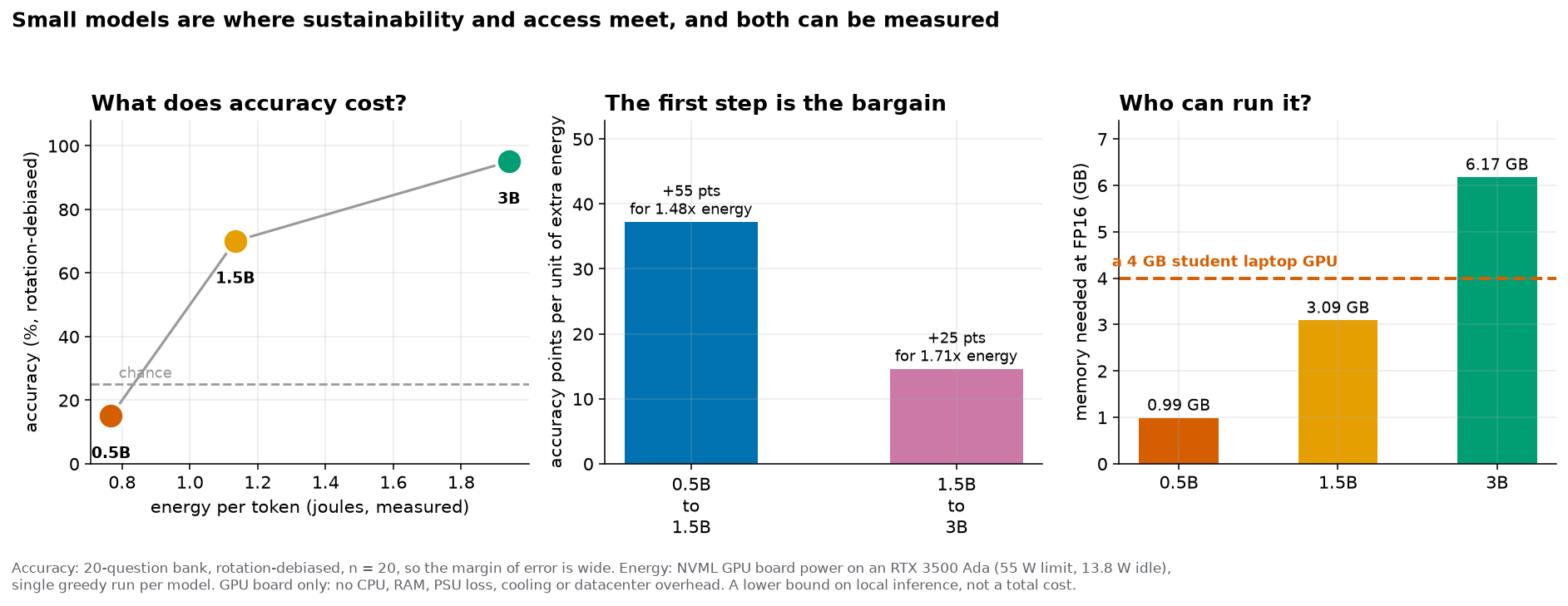
both can be measured". The left panel, “What does accuracy cost?”, plots accuracy from 0 to 100 percent on the vertical axis against measured energy per token in joules from about 0.7 to 1.9 on the horizontal axis. Three dots joined by a grey line rise steeply then flatten: 0.5B at about 0.77 joules and 15 percent, 1.5B at about 1.13 joules and 70 percent, and 3B at about 1.94 joules and 95 percent. A dashed grey line marks chance at 25 percent, above the 0.5B dot. The middle panel, “The first step is the bargain”, has two bars showing accuracy points per unit of extra energy: the 0.5B to 1.5B step reaches about 37 and is labelled plus 55 points for 1.48 times energy, and the 1.5B to 3B step reaches about 15 and is labelled plus 25 points for 1.71 times energy. The right panel, “Who can run it?”, has three bars of memory needed at FP16, 0.99, 3.09 and 6.17 gigabytes, with a dashed orange line at 4 gigabytes labelled “a 4 GB student laptop GPU”. The first two bars are below the line and the third is above it. :name: fig-ch07-theme-s :width: 100%
The two factors, measured on the same three models. Accuracy is rotation-debiased on a
twenty-question bank, so the margin of error is wide; the finding is the shape, not the exact
percentages. Energy is NVML GPU board power on an RTX 3500 Ada with a 55 W limit and 13.8 W idle,
one greedy run per model, GPU board only, with no CPU, RAM, power-supply losses, cooling or
datacentre overhead. Produced by lab/fig_theme_s.py from lab/out/lab4_size_ladder.json and
lab/out/theme_s_energy.json.
Move the slider in the simulation below to the memory your own machine has, and watch the ceiling move.
Every definition in this chapter, in one place
| # | Term | One line |
|---|---|---|
| 7.1 | Quantization | Rounding each weight to one of a small set of allowed levels and storing which one. |
| 7.2 | Bit | One binary digit. With bits you can name things. |
| 7.3 | Scale | The gap between two neighbouring levels. Multiply a stored level by it to get a weight. |
| 7.4 | Per-tensor quantization | One scale for every weight in a tensor. The naive method. |
| 7.5 | Quantize and dequantize | Divide by the scale and round; then multiply back by the scale. |
| 7.6 | Rounding error | The gap between the original weight and the one that comes back. Never more than half a scale. |
| 7.7 | Outlier | A weight far larger in size than the typical weight in the same tensor. |
| 7.8 | Block | A short run of consecutive weights sharing one scale. here. |
| 7.9 | Blockwise quantization | One scale per block, sized by that block’s own largest weight. |
| 7.10 | Watt, joule, watt-hour | A rate of energy; a unit of energy; one watt for an hour, or 3,600 joules. |
| 7.11 | Board power and idle power | What the whole card draws; what it draws with nothing running. |
| 7.12 | Accuracy points per unit of extra energy | Points gained by a step, divided by the energy multiple that step costs. |
The twelve formulas of this chapter, collected
| # | Name | The formula | Used for |
|---|---|---|---|
| 1 | Whole steps per side | how many marks the ruler gets | |
| 2 | The scale | how far apart the marks are | |
| 3 | Quantize, dequantize | , | what happens to one weight |
| 4 | Outlier ratio | diagnosing why per-tensor fails | |
| 5 | Relative error | mean divided by | reporting damage honestly |
| 6 | Blockwise scale | the fix | |
| 7 | Bytes per weight | what the fix costs | |
| 8 | File size | bytes per weight | what you download |
| 9 | Energy per token | what a token costs | |
| 10 | Watt-hours per 1,000 tokens | putting it in bill units | |
| 11 | Energy above idle | the marginal cost | |
| 12 | Points per unit of energy | which step is the bargain |
A thirteenth formula is used in Section 7.4 and is not counted among the twelve, because it is not a quantization formula. It is the standard deviation, , which Formula 5 divides by. It is set out in full immediately before Formula 5, and again in the Math Toolkit.
Every one of these is also in the formula summary appendix, with a second worked example.
Common mistakes
These are the eight things that actually go wrong, in the order they tend to go wrong.
Computing instead of . At 4 bits that gives 15 steps instead of 7, so every scale afterwards comes out a little under half the size it should be: where the right answer is 0.17522321. How to spot it: divide the largest weight by your scale. You must land exactly on the number of steps. At 4 bits that is 7. If you land on 15, this is your error.
Rounding before dividing. Formula 3 divides the weight by the scale first, then rounds. Rounding the weight and then dividing gives nonsense. How to spot it: your stored value will not be a whole number, or it will be wildly outside the range -7 to +7.
Believing more bits always help one particular weight. They help on average, over many weights. On a single chosen weight the error depends on where it lands between two marks, and Cell 7 in this chapter shows a 4-bit error larger than the 3-bit error on the same weight. How to spot it: you are comparing one weight, not a mean.
Forgetting the block scales when counting storage. “4-bit” costs 0.5 bytes per weight only if the scales are free, and they are not. The honest figure is 0.5625. How to spot it: your model size comes out as 0.247 GB where the honest answer is 0.278 GB. Be careful which way round you state that gap. The scales add 12.5% on top of 0.247, since . They are not 12.5% of 0.278. The toolkit on percentage points is where this trap is set out in full.
Saying “4-bit loses 25% of the quality”. Four bits is not a method. On this matrix, four bits gave 46.6% weight error one way and 7.2% the other way. And weight error is not quality; quality needs a named test with a named number of questions. How to spot it: the claim has a bit count and no scheme, or a quality figure and no test.
Confusing watts with joules. A watt is a rate and a joule is an amount. “The card used 21 watts” does not say how much energy anything cost until you also say for how long. How to spot it: your energy figure has no time in it anywhere.
Quoting the energy figures as a total cost. They are GPU board power only. No processor, no memory, no power supply losses, no cooling, no building. They are a lower bound. How to spot it: you wrote “a token costs 0.767 joules” without the words “at the graphics card”.
Treating 15%, 70% and 95% as precise. Each is twenty questions. The ordering and the rough size of the steps are the finding; the exact percentages are not. How to spot it: you quoted a difference of a few points as though it were meaningful. On twenty questions, even a 25-point difference is not statistically significant, as Chapter 13 shows.
What to remember
Quantization is rounding every weight to one of a short list of allowed values, and the gap between those values, the scale, is set by the largest weight sharing it. In a real attention matrix the largest weight is about 45 times the typical one, so one scale for the whole matrix erases the median weight at 4 bits and throws away 46.6% of the weights’ spread. Giving each run of 32 weights its own scale drops that to 7.2% for 12.5% more storage, which is what real quantizers in GGUF do. The same shrinking that makes a model cheap in bytes makes it cheap in joules and possible on a modest machine: 0.767, 1.133 and 1.941 joules per token, and 0.99, 3.09 and 6.17 gigabytes, for the three models this course uses. Both of those measurements, taken separately and for different reasons, point at the same model, and that is what this course means when it says sustainability and access are one variable seen twice.
Practice problems
Thirty problems in three tiers. Warm-up checks the arithmetic. Practice asks you to apply it. Stretch asks you to reason with it and, in several cases, to say what cannot be concluded. Answers to the odd-numbered problems are in the answers appendix.
Where a problem uses the real matrix, the numbers you need are: largest weight size 1.2265625, median weight size 0.02697754, standard deviation 0.066741, and weights. Where a problem uses the models, the numbers are in the tables in Sections 7.7 and 7.8.
Warm-up
How many whole steps sit on each side of zero at bits? Show the two steps of Formula 1.
How many whole steps at bits? At bits?
Compute the per-tensor scale at 6 bits for the real matrix, using . Check your answer by multiplying back.
Compute the per-tensor scale at 3 bits for the same matrix.
Quantize and dequantize the weight at 6 bits per-tensor. Give , the rounded , the value that comes back, and the error.
A weight is and the scale is . Find , find , and find the error.
Compute the outlier ratio for the real matrix from the largest and median sizes given above. Round to two decimal places.
A block of four weights is 0.06, -0.04, 0.01, 0.02. What is the largest size in the block? What is the block scale at 4 bits?
Convert 4.5 bits per weight into bytes per weight. Then convert 6 bits per weight into bytes per weight.
A scheme uses 3-bit weights with one 16-bit scale per 32 weights. How many bits per weight is that, and how many bytes?
How many joules does the 1.5B model spend on 250 tokens, at 1.133 joules per token?
Convert 1.133 joules per token into watt-hours per 1,000 tokens, using Formula 10.
The 3B model averaged 30.203 watts for 5.6539 seconds. How many joules is that in total?
Practice
Work out the full per-tensor scale table for the real matrix at and check that each scale is larger than the one above it. Explain in one sentence why that ordering is guaranteed.
At 4 bits per-tensor on the real matrix, any weight smaller in size than half the scale rounds to zero. Compute that threshold. Then say whether weights of size 0.05, 0.09 and 0.20 survive.
Take the four made-up weights 0.12, -0.07, 0.04, -0.02. Quantize and dequantize them at 4 bits per-tensor, using , and compute the mean absolute error.
Take the same four weights and quantize them at 4 bits blockwise, treating them as one block. Compute the block scale, the four dequantized values, and the mean absolute error. How many times better is the blockwise result?
Using your answers to 16 and 17, compute the standard deviation of the four original weights and express both mean errors as a percentage of it, following Formula 5.
A scheme stores weights at 2 bits with one 16-bit scale per 16 weights. Compute the bits per weight, the bytes per weight, and the size of the 0.5B model under it. Then say why a smaller block makes the overhead worse.
The 0.5B model at FP16 is 0.988 GB, and at 4-bit blockwise it is 0.278 GB. By what factor did the file shrink? Apply the same factor to the 3B model’s 6.17 GB and say what you get, then say why that result is arithmetic and not a measurement.
Using Formula 11 and the figures W, W, s and tokens, compute the joules per token above idle for the 1.5B model. Then compute what share that is of its full 1.133 joules per token.
A student generates 20,000 tokens over a semester on the 1.5B model. How many watt-hours is that at the graphics card? How many seconds of a 60 watt bulb?
Apply Formula 12 to both steps of the ladder, showing all three steps of arithmetic each time, and state which step is the better bargain and by what factor.
Stretch
Someone proposes fixing the per-tensor problem by clipping: before quantizing, replace any weight larger in size than 0.2 with 0.2, then set the scale from the clipped matrix. Work out the new 4-bit scale. Say what this buys and what it costs, and name the group of weights that pays the price.
Blockwise quantization with needs 25,088 scales for this one matrix. Suppose you used instead. Compute the bits per weight and the model size, and argue both sides of whether the smaller block is worth it. What measurement would settle it?
In Cell 7 the blockwise error on the typical weight was 0.00535366 at 4 bits and 0.00174967 at 3 bits, so the 3-bit result was better for that one weight. Explain why this is not a contradiction of the claim that more bits are better, and describe an experiment with this chapter’s code that would show your explanation is right.
This chapter reports weight error and not answer quality. Write a short paragraph explaining the difference, then design an experiment that would measure answer quality after quantization. Say how many questions you would use and why, referring to what Chapters 12 and 13 establish about small question banks.
The energy figures are GPU board power only. Suppose you were asked to produce a total cost of ownership figure for running the 1.5B model on a laptop for a year. List every quantity you would need to measure or find, mark each one as measurable with the equipment in this course or not, and say what you would write in the report for the ones you could not measure.
The course’s claim is that the energy argument and the access argument point at the same model. Describe a situation in which they would point at different models, be specific about what would have to be true of the hardware or the measurements, and say what you would do about it.
A vendor publishes a chart showing their 4-bit quantized model at 98% of the original model’s accuracy. Using this chapter and the warnings in it, list the five questions you would ask before accepting that chart, and for each one say what answer would satisfy you.
Where this goes next
Chapter 8 leaves precision behind and starts on geometry: what it means to say two sentences are close together. The quantization thread returns in Lab 1, where you measure size, speed, quality and energy on a model you shrink yourself, and it returns again in Chapter 14, where the question stops being what a token costs and becomes who pays.