Retrieval: the open-book exam - Inside the Machine: The Mathematics of Small Language Models

Chapter 10. Retrieval: the open-book exam

What you need before this chapter¶

This chapter is the payoff of the two before it. Almost everything it needs, you already built.

From this book.

Chapter 8, A sentence is an arrow. A piece of text becomes a list of numbers. That list is called an embedding, and you can treat it as an arrow.
Chapter 9, Similarity is geometry. Two arrows are compared by cosine similarity: their dot product divided by both of their lengths. The answer runs from -1 to 1.

If either of those is hazy, read Chapter 9’s first two sections again before starting here. This chapter uses cosine similarity on every page. It does restate the formula in full below, so you are not stranded, but it moves faster than Chapter 9 did.

From the Math Toolkit. Every symbol this chapter uses is explained from zero on that page.

You will meet	Toolkit section
A letter standing for a number	Section 1
Subscripts, such as $d_3$ and $s_{(2)}$	Section 2
Multiplication, written four ways	Section 3
The fraction bar as division, and the $\div$ sign	Section 4
Square roots, used inside the length of a vector	Section 9
$\sum$ , the instruction to add a list up, and the bar that means “average”	Section 10
Percentages, decimals and fractions	Section 11
Percentage points, which are not the same as percent	Section 11
Proportions, and what “3 out of 6” means	Section 12
Reading a bar chart	Section 13
Coordinates, vectors, and the dot product	Section 14
Vector length, written with double bars	Section 15
Rounding and decimal places	Section 16
Inequality signs, such as $0.014 < 0.038$	Section 19

From the Python Reference. The code in this chapter needs two libraries installed, numpy and sentence-transformers. If either import fails, or if you have not set Python up at all, Section 2 of the Python Reference walks through it for Windows, macOS and Linux. Three more sections of that page are the exact moves this chapter makes: embedding sentences, normalising a vector, and computing a cosine similarity matrix.

What you do not need. You do not need to know how an embedding model is trained. You do not need calculus. You do not need to have written code before. Every line of Python below is printed, commented, and explained after it runs.

Setup¶

This is the whole software stack for the chapter. Run it once, at the top, and leave it alone.

# ---------------------------------------------------------------------------
# Setup for Chapter 10. One import per line, with a note on what each is for.
# ---------------------------------------------------------------------------

import os            # lets Python read and change settings on your computer
os.environ["HF_HOME"] = r"C:\math3219\models"   # where the models are kept; MUST come before the next import

import re            # finds patterns in text; used to tidy up a PDF-to-text file
import numpy         # holds long lists of numbers and multiplies them quickly

from sentence_transformers import SentenceTransformer   # turns a sentence into a list of numbers

# Where this course keeps its measured results. Every number printed in this
# chapter can be checked against a file in this folder.
LAB_OUTPUT_FOLDER = "lab/out"

print("setup finished")

That prints one line.

setup finished

SentenceTransformer is the only piece that is new. It is the tool that does the job of Chapter 8: hand it a sentence, get back a list of numbers.

A question nobody in the building can answer quickly¶

It is the second week of registration. A student is standing in the advising line in the Student Services building at CSU Bakersfield, holding a printout of a degree plan. They need one more course. They have found one that looks perfect and they want to know a single thing: does it count?

The rule that answers them is real, it is written down, and it is public. CSUB publishes a document called the GE Compendium, and one line inside it says:

“A course satisfying only (a) General Education requirement(s) must end in ‘9’ (xxx9).”

Another line, in the section on Area 2, says:

“The course must be lower division and open to all students.”

Those two sentences settle the student’s question. They are also buried in an eleven-thousand-word document that almost nobody reads end to end, which is part of why the line in Student Services exists at all.

So the student does what people now do. They open a chatbot and type the question.

Here is the problem. The model on the other end has never read CSUB’s GE Compendium. It was trained on a great deal of text, and the internal rules of one campus in Kern County were almost certainly not in it. The model will answer anyway. Chapter 4 explains exactly why. The only thing a language model does is produce a probability for every possible next token, and it will always produce one. There is no token for “I have not read that document.”

The fix is not a bigger model. The fix is to hand the model the page.

That is this chapter. You take the question, search the document for the passage most likely to hold the answer, and paste that passage into the prompt before the model writes a word. The exam stops being a memory test and becomes an open-book exam. The technique has a name, retrieval-augmented generation, usually shortened to RAG, and the searching half of it is something you already know how to do: turn everything into arrows, then find the arrow closest to the question.

Two things make this chapter more than a demonstration. First, the search is arithmetic you can do by hand, and you will do it by hand. Second, and this is the part most courses skip, the search fails, in ways you can diagnose. Half of this chapter is a real system failing twice before it worked, on a real CSUB document, with the numbers printed at each attempt.

Where every number in this chapter comes from

Two experiments, both run on the machine described in the lab notebook, both saved to disk.

The six-sentence example comes from lab/we5_embeddings.py, saved in lab/out/we5_embeddings.json. Six short sentences, one question, one embedding model called all-MiniLM-L6-v2, which produces 384 numbers per sentence. That 384 is the dim field of lab/out/we5_embeddings.json. The model’s parameter count, 22,713,216, is not in that file. It was counted by lab/lab2_rag_v3.py and stored in lab/out/lab2_rag_v3.json, and that is the file this chapter names every time it prints that number.

The three-pass story comes from lab/lab2_rag_corpus.py, lab/lab2_rag_v2.py and lab/lab2_rag_v3.py, saved in lab/out/lab2_rag.json, lab/out/lab2_rag_v2.json and lab/out/lab2_rag_v3.json. The corpus is CSUB’s own GE Compendium and the Cal-GETC Guiding Notes. Those are real documents you can open and check yourself, and that checkability is the whole reason for using them. A retrieval demonstration over invented documents cannot teach you whether retrieval worked.

Some worked examples on this page use small invented numbers such as $(3, 4)$ , because 3 and 4 are easier to check on a phone than 0.9101471900939941. Those are labelled made up for practice every time. A number labelled real is a number a script computed, and the file that holds it is named.

The book’s rule: we never publish a number we did not compute. Where a number does not exist, this chapter says so out loud rather than filling the gap with something plausible. There is one such place in this chapter, in Section 10.4, and it is marked.

Learning objectives¶

By the end of this chapter you will be able to:

Explain what retrieval does, in plain words, and say why handing a model a passage is a different operation from training a model on a document.
Compute a cosine similarity between a question and a passage by hand, rank a small set of passages by that score, and pick the nearest neighbour.
Compute and interpret the confidence gap, meaning the rank-1 score minus the rank-2 score, and explain why the gap rather than the top score is what tells you retrieval worked.
Diagnose a failed retrieval by reading what came back, and say whether the fault lies in the chunking, in the embedding model, or in the question.
Explain, using this course’s own measured results, why a diagnostic number is a property of the procedure that produced it and cannot be carried across to a different system.

This lesson at a glance¶

Retrieval is nearest neighbour. Turn the question into a list of numbers, turn every passage into a list of numbers, score each passage against the question with cosine similarity, and take the highest. That is the entire method.
The gap is the idea, not the top score. In the measured six-sentence run the two relevant sentences scored 0.910 and 0.719 and the best irrelevant one scored 0.089. The drop of 0.630 between rank 2 and rank 3 is what makes retrieval usable.
On a real document it failed twice. Fixed 120-word windows over the GE Compendium and the Guiding Notes returned the wrong section. Heading-aware chunks over the Compendium got 3 questions of 6. Only a different embedding model got 6 of 6.
The sting. The system that scored 6 of 6 had a mean confidence gap of 0.055, which is lower than the 0.058 of the system that scored 3 of 6. A gap is a useful signal inside one system and does not transfer between systems.

The vocabulary of this chapter¶

Every term below is used later on this page. They are collected here first so that no sentence in this chapter depends on a word you have not met.

Term	In one line
Corpus	The collection of documents you are searching. More than one: corpora.
Passage	One piece of text out of the corpus, short enough to paste into a prompt.
Chunk	The same thing as a passage, named for how it was made: the document was cut into chunks.
Chunking	The act of cutting a long document into passages. It is a choice, and half of this chapter is about how much that choice changes the result.
Fixed-window chunking	Cutting every 120 words, regardless of what the document says. The simplest possible rule.
Overlap	Repeating the last few words of one chunk at the start of the next, so a sentence cut in half still appears whole somewhere.
Heading-aware chunking	Cutting at the document’s own headings, and gluing the heading onto the front of each chunk so the chunk carries a record of where it lives.
Query	The question, treated as a piece of text to be turned into numbers like any other.
Embedding	The list of numbers a model produces to stand for a piece of text. Here, 384 numbers.
Embedding model	The model that produces embeddings. Not the same model that writes the answer, and usually far smaller.
Dot product	Multiply two lists of numbers position by position, then add the products. The answer is one number.
Cosine similarity	The dot product divided by both lengths. Runs from -1 to 1 and depends only on direction.
Unit vector	A list of numbers whose length is exactly 1. Shrinking a list to length 1 is called normalising it.
Rank	Position in the sorted list of scores. Rank 1 is the highest score.
Order statistic	A score named by its rank instead of by which passage owns it. Written $s_{(1)}$ for the largest, $s_{(2)}$ for the next.
Nearest neighbour	The passage at rank 1, the one with the highest similarity to the query.
Top-k	The first $k$ passages in rank order. These are the ones you paste into the prompt.
The cut	The line between the last passage you keep and the first one you drop.
Confidence gap	The rank-1 score minus the rank-2 score. Large means the winner won by a wide margin.
Mean gap	The average confidence gap across a set of questions. One number summarising a whole run.
Hits at rank 1	The share of $n$ questions that put the correct passage first: the count that came back right, divided by $n$ . Written `hits@1`.
Sample proportion	A count of successes divided by the number of tries. `hits@1` is one. So is a model’s score on a test, in Chapter 11.
Semantic attractor	A chunk that keeps winning questions it should lose, because its wording resembles many questions at once.
Query prefix	A fixed phrase that some embedding models expect on the front of the question and nowhere else, because that is how they were trained.
RAG	Retrieval-augmented generation. Search the corpus, paste what you find into the prompt, then let the model answer.
Context length	The largest number of tokens a model can hold at once. It is the reason you cannot paste the whole document in and skip retrieval.

10.1 Scoring every passage against the question¶

Intuition¶

Think about how you actually use an index at the back of a book. You do not read the book. You look up a word, you turn to the page it points at, and you read half a page. The index is a device for turning a question into a location.

An index has one weakness, and everyone who has ever used one has met it. The index only knows the words the author chose to list. If you want to know about “the cost of running a model” and the author indexed it under “inference expense”, the index is silent. It matches letters, not meaning.

Retrieval is an index that matches meaning instead of letters. Here is the whole idea in four steps.

Cut the document into short passages.
Turn every passage into a list of numbers, using the embedding model from Chapter 8. Passages about similar things end up with similar lists.
Turn the question into a list of numbers the same way, with the same model.
Score the question’s list against every passage’s list, using cosine similarity from Chapter 9. Take the highest.

Step 4 is where the index’s weakness disappears. The question and the passage do not have to share a single word. In the lab’s measured run, two sentences with no content words in common, “The cat sat on the mat” and “A kitten rested on the rug”, scored 0.612 against each other (real, from lab/out/we5_embeddings.json). No index built on letters could connect those.

Nothing here understands anything. That sentence is worth reading twice. There is no comprehension in the machine at step 4. There is a list of numbers for the question, a list of numbers for each passage, a multiplication, an addition and a division. The result is a ranking. Everything this chapter calls “finding the right passage” is that ranking coming out in a helpful order, and the rest of the chapter is about the times it does not.

One more practical reason retrieval exists. A model can only hold so much text at once. That limit is called the context length, and it is counted in tokens, not words. You cannot paste an eleven-thousand-word document into a prompt and let the model sort it out. You have to choose what to send. Retrieval is the choosing.

The mathematics¶

Three formulas do all the work in this section. The first two you have met; they are restated here in full because this chapter leans on them.

Formula 10.1: Cosine similarity¶

In words. Two pieces of text each become a list of numbers. To score how alike they are, multiply the matching numbers and add up all the products, then divide by the length of the first list multiplied by the length of the second. That division removes the effect of size and leaves only direction, which is what you want, because a longer passage should not count as a better match for being longer.

The formula.

\cos(\mathbf{q}, \mathbf{d}) = \frac{\mathbf{q} \cdot \mathbf{d}} {\lVert \mathbf{q} \rVert \; \lVert \mathbf{d} \rVert}

The symbols.

Symbol	How to say it out loud	What it means
$\mathbf{q}$	“bold q”	the embedding of the query. Bold type means this is a whole list of numbers, not one number.
$\mathbf{d}$	“bold d”	the embedding of one passage. The letter $d$ is for “document”.
$\cos(\mathbf{q}, \mathbf{d})$	“cosine of q and d”	the answer: one number between -1 and 1
the minus sign in -1	“minus one”, or “negative one”	here the minus sign is not an instruction to subtract. It marks a number as sitting below zero, the way a temperature below freezing does. So the answer can be anywhere from one below zero up to one above it.
the round brackets and the comma	“of ... and ...”	they hold the two things the answer depends on. They do not mean multiply.
$=$	“equals”	the two sides are the same number
$\cdot$	“dot”	the dot product. Between two bold letters this raised dot means the whole multiply-and-add procedure, not ordinary multiplication.
$\lVert \mathbf{q} \rVert$	“the length of q”	how long that arrow is. Double upright bars mean length. Single bars would mean absolute value, which is a different thing.
$\lVert \mathbf{d} \rVert$	“the length of d”	the length of the other arrow
the space between the two lengths	“times”	multiply the two lengths together
the fraction bar	“divided by”	divide everything on top by everything underneath
$\times$	“times”	ordinary multiplication between two single numbers, as in $3 \times 4 = 12$ . Written four ways in this book, all meaning the same thing. See Toolkit Section 3.
$\div$	“divided by”	ordinary division between two single numbers, as in $12 \div 4 = 3$ . It does the same job as the fraction bar, written along one line instead of stacked. The worked examples below use it, and it is the key marked $\div$ on a phone calculator. See Toolkit Section 4.
$\sqrt{\phantom{n}}$	“the square root of”	the tick-with-a-roof sign. It appears in the worked example below, not in the formula itself, because finding a length needs it. “The square root of 25” means the number that gives 25 when multiplied by itself, which is 5, because $5 \times 5 = 25$ . See Toolkit Section 9.
“square each number”	“square”	multiply a number by itself. Squaring 3 means $3 \times 3 = 9$ . It is the undoing of a square root.

Out loud. “The cosine similarity of the query and a passage is their dot product, divided by the length of the query times the length of the passage.”

Worked, with numbers made up for practice. Real embeddings have 384 numbers each, which is too many to check by hand, so take two numbers each instead. The arithmetic is identical; there is less of it. Let the query be $\mathbf{q} = (3, 4)$ and the passage be $\mathbf{d} = (4, 3)$ .

Step 1, the dot product. Multiply the first numbers together, multiply the second numbers together, then add. $3 \times 4 = 12$ $4 \times 3 = 12$ $12 + 12 = 24$

Step 2, the length of the query. Square each number, add, take the square root. $3 \times 3 = 9$ $4 \times 4 = 16$ $9 + 16 = 25$ $\sqrt{25} = 5$

Step 3, the length of the passage. Same procedure. $4 \times 4 = 16$ $3 \times 3 = 9$ $16 + 9 = 25$ $\sqrt{25} = 5$

Step 4, multiply the two lengths. $5 \times 5 = 25$

Step 5, divide the dot product by that. $24 \div 25 = 0.96$

\cos(\mathbf{q}, \mathbf{d}) = 0.96

Check it. The answer must land between -1 and 1. If yours did not, the most likely slip is forgetting a square root in Step 2 or Step 3. A second check: the answer should not change if you make one of the lists longer without turning it. Try $\mathbf{d} = (8, 6)$ , which is $(4,3)$ doubled. Dot product: $3 \times 8 = 24$ , then $4 \times 6 = 24$ , then $24 + 24 = 48$ . The query’s length is still 5. The new passage’s length is $8 \times 8 = 64$ , then $6 \times 6 = 36$ , then $64 + 36 = 100$ , then $\sqrt{100} = 10$ . Multiply the lengths: $5 \times 10 = 50$ . And $48 \div 50 = 0.96$ , the same answer. Length is not meaning.

Formula 10.2: When both lists have length 1, cosine is the dot product¶

In words. If you shrink every list in advance so that its length is exactly 1, then the dividing step divides by 1, and dividing by 1 changes nothing. So you can skip it. The dot product on its own is then already the cosine similarity. Software does this because it makes the search much faster, and it is the reason the code below never appears to divide by anything.

The formula.

\text{if } \lVert \mathbf{q} \rVert = 1 \text{ and } \lVert \mathbf{d} \rVert = 1, \quad \text{then} \quad \cos(\mathbf{q}, \mathbf{d}) = \mathbf{q} \cdot \mathbf{d}

The symbols.

Symbol	How to say it out loud	What it means
“if” and “then”	“if”, “then”	ordinary English, doing ordinary English work. The statement on the right is only true when the condition on the left holds.
$\lVert \mathbf{q} \rVert = 1$	“the length of q equals one”	the arrow has been shrunk until it is exactly one unit long. A list like this is called a unit vector.
$\text{and}$	“and”	both conditions have to hold, not one of them
$\quad$	no sound	blank space, used to stop the two halves crowding each other
$\cos(\mathbf{q}, \mathbf{d})$	“cosine of q and d”	the same quantity as in Formula 10.1
$\mathbf{q} \cdot \mathbf{d}$	“q dot d”	the dot product, with no division after it

Out loud. “If both lists have been shrunk to length one, then the cosine similarity is the dot product.”

Worked, with numbers made up for practice. Take the same two lists as before, $\mathbf{q} = (3, 4)$ and $\mathbf{d} = (4, 3)$ , and shrink each to length 1 first.

Step 1, shrink the query. Its length is 5, from Step 2 of the previous worked example. Divide every number in it by 5. $3 \div 5 = 0.6$ $4 \div 5 = 0.8$ The shrunk query is $(0.6,\; 0.8)$ .

Step 2, check that it really has length 1. $0.6 \times 0.6 = 0.36$ $0.8 \times 0.8 = 0.64$ $0.36 + 0.64 = 1.00$ $\sqrt{1.00} = 1$

Step 3, shrink the passage. Its length is also 5. $4 \div 5 = 0.8$ $3 \div 5 = 0.6$ The shrunk passage is $(0.8,\; 0.6)$ .

Step 4, take the dot product of the two shrunk lists, and do not divide by anything. $0.6 \times 0.8 = 0.48$ $0.8 \times 0.6 = 0.48$ $0.48 + 0.48 = 0.96$

\mathbf{q} \cdot \mathbf{d} = 0.96

That is the same 0.96 as Formula 10.1 gave, reached with two multiplications and one addition instead of a square root and a division.

Check it. A unit vector dotted with itself gives exactly 1, because that is what “length 1” means. Test it on the shrunk query: $0.6 \times 0.6 + 0.8 \times 0.8 = 0.36 + 0.64 = 1.00$ . If you get something other than 1, the shrinking went wrong. The usual slip is dividing by the sum of the numbers, $3 + 4 = 7$ , instead of by the length, $\sqrt{3 \times 3 + 4 \times 4} = \sqrt{9 + 16} = \sqrt{25} = 5$ .

Formula 10.3: The retrieval rule¶

In words. Score the question against every passage in the collection, one at a time, and hand back whichever passage scored highest.

The formula.

\text{best passage} = \arg\max_{k \in \{1, \ldots, N\}} \; \cos(\mathbf{q}, \mathbf{d}_k)

The symbols.

Symbol	How to say it out loud	What it means
$\text{best passage}$	“best passage”	the answer. It is a passage, not a score.
$=$	“equals”	the two sides are the same thing
$\arg\max$	“arg max”	“the one that makes what follows biggest”. $\max$ hands you the biggest score; $\arg\max$ hands you which passage got it.
the small print under $\arg\max$	“over”	everything written below the words “arg max” says which candidates are allowed into the contest. It is not part of the score. Read it as “looking over all of these”.
$k$	“kay”	a counter over the passages. $k = 1$ is the first passage, $k = 2$ the second.
$\in$	“in”	“is a member of”. It says which values $k$ is allowed to take.
$\{1, \ldots, N\}$	“the set one through capital N”	curly brackets hold a set, a collection of allowed values. Here: every whole number from 1 to $N$ .
$\ldots$	“and so on”	keep counting in the same pattern
$N$	“capital N”	how many passages are in the corpus. In this chapter it is 6, then 248, then 77.
the blank space after the set	no sound	spacing only, keeping the two halves of the line from crowding each other
$\mathbf{d}_k$	“bold d sub k”	the embedding of passage number $k$ . The little $k$ written below the line is a subscript, and it says which passage. See Toolkit Section 2.
$\cos(\mathbf{q}, \mathbf{d}_k)$	“cosine of q and d sub k”	the score from Formula 10.1, between the query and passage $k$

Out loud. “The best passage is the one, out of all $N$ of them, whose embedding has the largest cosine similarity with the question’s embedding.”

Worked, with numbers made up for practice. The query is $\mathbf{q} = (3, 4)$ and there are three passages, so $N = 3$ : $\mathbf{d}_1 = (4, 3)$ , $\mathbf{d}_2 = (-4, 3)$ , $\mathbf{d}_3 = (6, 8)$ .

The second passage has a minus sign in front of its first number, so two rules about minus signs are needed before the arithmetic starts. A positive number times a negative number gives a negative answer: $3 \times (-4) = -12$ . A negative number times itself gives a positive answer: $(-4) \times (-4) = 16$ . The two minus signs cancel each other out.

Step 1, score passage 1. This is the same pair as Formula 10.1, so the working is repeated here rather than pointed at. Dot product: $3 \times 4 = 12$ , then $4 \times 3 = 12$ , then $12 + 12 = 24$ . Length of $\mathbf{q}$ : $3 \times 3 = 9$ , then $4 \times 4 = 16$ , then $9 + 16 = 25$ , then $\sqrt{25} = 5$ . Length of $\mathbf{d}_1$ : $4 \times 4 = 16$ , then $3 \times 3 = 9$ , then $16 + 9 = 25$ , then $\sqrt{25} = 5$ . Multiply the lengths: $5 \times 5 = 25$ . Divide: $24 \div 25 = 0.9600$ .

Step 2, score passage 2. Dot product: $3 \times (-4) = -12$ , then $4 \times 3 = 12$ , then $-12 + 12 = 0$ . Adding 12 to -12 lands exactly on zero. Length of $\mathbf{q}$ : 5, computed in Step 1 and unchanged, because the query has not moved. Length of $\mathbf{d}_2$ : $(-4) \times (-4) = 16$ , then $3 \times 3 = 9$ , then $16 + 9 = 25$ , then $\sqrt{25} = 5$ . The minus sign has disappeared, which is the point of the second rule above: length is never negative. Multiply the lengths: $5 \times 5 = 25$ . Divide: $0 \div 25 = 0.0000$ .

Step 3, score passage 3. Dot product: $3 \times 6 = 18$ , then $4 \times 8 = 32$ , then $18 + 32 = 50$ . Length of $\mathbf{q}$ : 5, again from Step 1. Length of $\mathbf{d}_3$ : $6 \times 6 = 36$ , then $8 \times 8 = 64$ , then $36 + 64 = 100$ , then $\sqrt{100} = 10$ , because $10 \times 10 = 100$ . Multiply the lengths: $5 \times 10 = 50$ . Divide: $50 \div 50 = 1.0000$ .

Step 4, compare the three scores and take the biggest. 0.9600, 0.0000, 1.0000. The biggest is 1.0000, which belongs to passage 3.

\text{best passage} = \mathbf{d}_3

Check it. The output of $\arg\max$ is an identity, not a size. If you wrote down 1.0000 you answered a different question; $\max$ gives the score, $\arg\max$ gives the passage. Two further checks: every individual score must sit between -1 and 1, and if two passages tie, the rule does not say which to take, so software picks one arbitrarily and you should treat a tie as a warning rather than an answer.

Python¶

Now do it on real text with a real model. The six sentences below are the exact six the lab used, in the exact order it used them, so every number printed here can be checked against lab/out/we5_embeddings.json.

# The six sentences the lab measured. They stay in this order for the whole chapter,
# so that "sentence 2" always means the same sentence.
six_sentences = []
six_sentences.append("The cat sat on the mat.")
six_sentences.append("A kitten rested on the rug.")
six_sentences.append("Bakersfield is in Kern County, California.")
six_sentences.append("Kern County's largest city is Bakersfield.")
six_sentences.append("The stock market fell sharply on Tuesday.")
six_sentences.append("Photosynthesis converts light into chemical energy.")

# Load the embedding model. The first run downloads it; later runs read it from
# disk. This is NOT the model that writes answers. It only measures meaning.
# It has 22,713,216 parameters (counted in lab/out/lab2_rag_v3.json) against the
# 494,032,768 of the 0.5B model from Chapter 3 (lab/out/theme_s_energy.json).
# Dividing one by the other: 494,032,768 / 22,713,216 = 21.7509, which rounds
# to 21.75, so the embedding model is about 22 times smaller.
embedding_model = SentenceTransformer("sentence-transformers/all-MiniLM-L6-v2")

# Turn all six sentences into lists of numbers.
# normalize_embeddings=True shrinks every list to length exactly 1, which is
# Formula 10.2: after this, a plain dot product IS the cosine similarity.
sentence_vectors = embedding_model.encode(six_sentences, normalize_embeddings=True)

print("how many sentences:", len(six_sentences))
print("shape of the block of numbers:", sentence_vectors.shape)

# numpy.linalg.norm measures the length of a list of numbers, which is the
# denominator of Formula 10.1. "%.6f" is a printing instruction, not arithmetic:
# it says "write this number with six digits after the decimal point".
print("length of row 0 after normalising: %.6f" % numpy.linalg.norm(sentence_vectors[0]))

That prints three lines.

how many sentences: 6
shape of the block of numbers: (6, 384)
length of row 0 after normalising: 1.000000

Read each line. The first says there are six sentences, which you already knew. The second is the one that matters: (6, 384) means the model handed back a block of numbers with 6 rows and 384 columns. One row per sentence, 384 numbers in each row. Those 384 numbers are the whole of what the machine will know about that sentence from here on. The sentence itself is never looked at again.

The third line is the check from Formula 10.2. Every row has been shrunk to length exactly 1, so for the rest of this chapter a dot product is a cosine similarity, and no division is needed.

Two details in that code are worth naming, because they are the two things students change first and break first. normalize_embeddings=True is not a formatting option. It is the arithmetic of Formula 10.2, and turning it off means every score from here on would need dividing by two lengths. And the query has to go through the same model as the passages. Two models produce two different sets of 384 numbers, and a cosine similarity between a list from one model and a list from another is a number with no meaning at all, even though the code will happily compute it and print something.

Try it 10.1: predict the shape

Suppose you added two more sentences to six_sentences, making eight, and ran the same code. What would the second line print? And suppose instead you swapped all-MiniLM-L6-v2 for a model that produces 768 numbers per sentence, keeping six sentences. What would it print then?

10.2 The gap is the whole idea¶

Intuition¶

Picture a hiring panel scoring six applicants out of 100. Two sets of scores follow. Both are made up for practice, and both are the sort of thing a panel really sees.

In the first, the scores are 91, 72, 9, 6, 6 and 1. Nobody on that panel needs a discussion. Two people are in a different category from the other four, and the winner is not in doubt.

In the second, the scores are 62, 61, 60, 60, 59 and 58. The top score is still the top score. The panel still has a ranking. But the ranking is telling them almost nothing, because a single point either way would rearrange the whole list. The right response is not “hire number one”. It is “our scoring method is not separating these people”.

A retrieval system hands you the first kind of result on easy material and the second kind on hard material, and it looks identical either way. It always returns a rank 1. It never tells you that rank 1 barely beat rank 2. If you only look at the winner, the two situations are indistinguishable.

So the number to look at is not the top score. It is the gap: how far rank 1 sits above rank 2. A large gap means the method found something. A small gap means the method ranked noise and handed you the top of the noise with a straight face.

This is the single most useful habit in the chapter, and it transfers well beyond retrieval. Whenever a procedure ranks things and hands you a winner, ask how far ahead the winner finished.

Here is the measured result. The lab put one question, “Which California county is Bakersfield in?”, against the six sentences from Section 10.1. The two sentences about Kern County scored 0.910 and 0.719. The best of the four irrelevant sentences scored 0.089. Between rank 2 and rank 3 the score falls off a cliff, and the cliff sits exactly where the relevant sentences run out. That cliff is retrieval working. Not the 0.910.

The mathematics¶

The gap needs one new piece of notation, and it is a small one.

Formula 10.4: The confidence gap¶

In words. Take the highest score. Subtract the second highest score. What is left tells you by how much the winner won.

The formula.

g = s_{(1)} - s_{(2)}

The symbols.

Symbol	How to say it out loud	What it means
$g$	“gee”	the answer: the confidence gap. A letter standing for a number, as in Toolkit Section 1.
$=$	“equals”	the two sides are the same number
$s$	“ess”	a similarity score. Every $s$ in this formula is a cosine similarity from Formula 10.1.
$s_{(1)}$	“s sub bracket one”	the largest score in the list, the one at rank 1
$s_{(2)}$	“s sub bracket two”	the second largest score, the one at rank 2
the round brackets in the subscript	no sound	they mark the number as a rank, not as a passage’s position in storage
$-$	“minus”	subtract the second from the first

Out loud. “The gap is the rank-one score minus the rank-two score.”

Worked, with real numbers. From lab/out/we5_embeddings.json, the six cosine similarities between the query “Which California county is Bakersfield in?” and the six sentences, sorted largest first and rounded to three decimal places:

Rank $r$	$s_{(r)}$	Sentence
1	0.910	Bakersfield is in Kern County, California.
2	0.719	Kern County’s largest city is Bakersfield.
3	0.089	The cat sat on the mat.
4	0.062	A kitten rested on the rug.
5	0.056	Photosynthesis converts light into chemical energy.
6	0.012	The stock market fell sharply on Tuesday.

Step 1, identify the rank-1 score. $s_{(1)} = 0.910$ .

Step 2, identify the rank-2 score. $s_{(2)} = 0.719$ .

Step 3, subtract. $0.910 - 0.719 = 0.191$

g = 0.191

Check it. The gap can never be negative. If you got a negative number, you subtracted the wrong way round or you did not sort first. The gap can also never be larger than 2, because every cosine sits between -1 and 1, so the largest possible difference is $1 - (-1) = 2$ . In practice, gaps this small in absolute size are normal and the number only means something relative to other gaps from the same system, which is a point Section 10.6 will make the hard way.

Worked example 10.1: the gap that actually matters here

The gap in Formula 10.4 compares rank 1 to rank 2. In this particular run, the interesting comparison is one step further down, between rank 2 and rank 3, because that is where the sentences about Kern County stop and the sentences about cats begin.

Step 1, the rank-2 score. $s_{(2)} = 0.719$ .

Step 2, the rank-3 score. $s_{(3)} = 0.089$ .

Step 3, subtract. $0.719 - 0.089 = 0.630$

Now compare the two drops.

Rank 1 to rank 2: 0.191.
Rank 2 to rank 3: 0.630.

The second drop is more than three times the first: $0.630 \div 0.191 = 3.30$ . The machine is telling you, in a number, that sentences 1 and 2 belong together and everything below them is a different kind of thing. Nothing told it that the first two sentences were about Kern County. It found the boundary by arithmetic.

All four values are real, from lab/out/we5_embeddings.json.

Python¶

The code below reproduces the table above. It scores the query against all six sentences, sorts them, and prints both the ranking and the drop between each rank and the next.

# The question. It is a piece of text like any other, and it goes through the
# same model as the six sentences did.
query_text = "Which California county is Bakersfield in?"

# Embed it, shrunk to length 1 like the others. encode() expects a list, so the
# question goes in as a list of one, and we take row 0 back out.
query_vector = embedding_model.encode([query_text], normalize_embeddings=True)[0]

# Score the question against every sentence. Because every list has length 1,
# a dot product IS the cosine similarity (Formula 10.2). The @ sign between two
# blocks of numbers is numpy's dot-product sign. It is the code spelling of the
# raised dot in Formula 10.1, and it has nothing to do with the @ in an email
# address. numpy does all six dot products in one line: the block of 6 rows
# against the single query row.
similarity_scores = sentence_vectors @ query_vector

# Sort the six positions from highest score to lowest.
# argsort sorts smallest-first, so we sort the negatives to get largest-first.
ranked_positions = numpy.argsort(-similarity_scores)

print("query:", query_text)
for rank_number in range(len(ranked_positions)):
    position = ranked_positions[rank_number]
    print("  rank %d  score=%.3f  %s" % (rank_number + 1,
                                         similarity_scores[position],
                                         six_sentences[position]))

That prints seven lines.

query: Which California county is Bakersfield in?
  rank 1  score=0.910  Bakersfield is in Kern County, California.
  rank 2  score=0.719  Kern County's largest city is Bakersfield.
  rank 3  score=0.089  The cat sat on the mat.
  rank 4  score=0.062  A kitten rested on the rug.
  rank 5  score=0.056  Photosynthesis converts light into chemical energy.
  rank 6  score=0.012  The stock market fell sharply on Tuesday.

Look at what the model was never told. It was never told that Kern County is in California. It was never told that Bakersfield is a city. It was never given a list of place names. It produced 384 numbers for each sentence and 384 numbers for the question, and the two Kern County sentences came out pointing in nearly the same direction as the question while the cat, the kitten, the stock market and the photosynthesis did not.

Notice also that rank 2 says almost the same thing as rank 1 in reversed word order, and scores 0.719 rather than 0.910. Word order and phrasing still move the number. Meaning is measured here, but it is measured roughly.

Now compute the drops. This is a second short cell so that the ranking above stays readable.

# The drop between each rank and the next one down. There are six scores, so
# there are five drops: 1 to 2, 2 to 3, 3 to 4, 4 to 5, 5 to 6.
print("drops between neighbouring ranks:")
for rank_number in range(len(ranked_positions) - 1):
    higher_position = ranked_positions[rank_number]
    lower_position = ranked_positions[rank_number + 1]
    drop = similarity_scores[higher_position] - similarity_scores[lower_position]
    print("  rank %d to rank %d:  %.3f" % (rank_number + 1, rank_number + 2, drop))

That prints six lines.

drops between neighbouring ranks:
  rank 1 to rank 2:  0.191
  rank 2 to rank 3:  0.630
  rank 3 to rank 4:  0.028
  rank 4 to rank 5:  0.006
  rank 5 to rank 6:  0.044

One of those five numbers is more than three times any of the other four, and it is the second one. The drop of 0.630 is the boundary between “about Kern County” and “not about Kern County”, found without anyone drawing that boundary.

The three drops below it, 0.028, 0.006 and 0.044, are worth a moment too. They do not shrink as you go down the list. The drop from rank 5 to rank 6 is larger than the drop from rank 3 to rank 4. Below the cliff, the ordering of the four irrelevant sentences is close to meaningless, and the small drops are the number telling you so.

Try it 10.2: read a ranking and judge it

A retrieval system is asked a question and returns five passages with these cosine similarities, already sorted. The five numbers are made up for practice; no script produced them.

0.412, \quad 0.406, \quad 0.399, \quad 0.395, \quad 0.390

(a) What is the confidence gap $g$ ? (b) Would you paste passage 1 into a prompt and let a model answer from it? (c) What would you do instead?

10.3 How much book to hand over¶

Intuition¶

Retrieval does not have to return one passage. Usually it returns several, and you paste all of them into the prompt before the question. The count has a name: $k$ . Taking the top three passages is “ $k = 3$ ”.

Choosing $k$ is a real trade-off with a cost on both sides.

Too small and you miss the answer. If the answer is split across two passages and you take one, the model gets half a rule. It will answer from the half it was given, confidently, and the answer will be wrong in a way that is hard to catch, because the sentence it produces will contain real words from a real document.

Too large and you bury it. Every extra passage is more tokens in the prompt. Three things get worse at once. The prompt costs more to process, which is the energy argument from Chapter 7 in a new costume. The model has a fixed context length and you are spending it. And the relevant passage is now surrounded by irrelevant text, which makes the model’s job harder rather than easier.

The six-sentence run makes the second cost visible. Send all six sentences and the model, in order to answer a question about a county, has to read about a cat, a kitten, the stock market and photosynthesis. Counting words: the six sentences hold 37 words in total, of which 25 belong to the four irrelevant sentences. Turn that into a percentage in two steps, the way Toolkit Section 11 does it. First divide the part by the whole: $25 \div 37 = 0.675675\ldots$ Then multiply by 100 to move from a decimal to a percentage: $0.675675 \times 100 = 67.5675$ , which rounds to 67.6. So 67.6% of the words you sent are noise, for a question with a two-sentence answer.

There is no formula that gives the right $k$ . There is a diagnostic, and it is the gap again, measured at the place you cut.

The mathematics¶

One warning about the letter $k$ before anything else, because it now does a second job. In Formula 10.3 the letter $k$ was a counter that walked through the passages one at a time, so $k = 1$ meant the first passage. From here on, $k$ means how many passages you send, so $k = 3$ means three passages. Same letter, different job. Reusing a letter this way is common in writing about retrieval, and the way to stay safe is to read the sentence around the letter rather than the letter alone. A letter carries no fixed meaning of its own, which is the point made in Toolkit Section 1.

Formula 10.5: The drop at the cut¶

In words. Pick how many passages you are going to send. Take the score of the last one you send and subtract the score of the first one you leave out. A big answer means you cut in a sensible place. A small answer means the passage you dropped was almost as good as the one you kept, so the cut was arbitrary.

The formula.

g_k = s_{(k)} - s_{(k+1)}

The symbols.

Symbol	How to say it out loud	What it means
$g_k$	“g sub k”	the answer: the drop at the cut, when you keep $k$ passages. The subscript says which cut you mean.
$=$	“equals”	the two sides are the same number
$k$	“kay”	how many passages you decided to send
$s_{(k)}$	“s sub bracket k”	the score at rank $k$ , the last passage you keep
$+$	“plus”	add. Here it adds 1 to a rank number to step one place down the list.
$k + 1$	“k plus one”	the next rank down
$s_{(k+1)}$	“s sub bracket k plus one”	the score at rank $k+1$ , the first passage you drop
the round brackets in the subscript	no sound	they mark the number as a rank, as in Formula 10.4, not as a passage’s position in storage
the small letters written below the line	“sub”	a subscript, which picks one item out of a list. See Toolkit Section 2.
$-$	“minus”	subtract

Out loud. “The drop at a cut of k is the score at rank k minus the score at rank k plus one.”

Formula 10.4 is the special case $k = 1$ : $g_1 = s_{(1)} - s_{(2)}$ , which is the confidence gap.

Worked, with real numbers. Using the six measured scores from Section 10.2, here is every possible cut.

Step 1, cut after 1. $g_1 = 0.910 - 0.719 = 0.191$ .

Step 2, cut after 2. $g_2 = 0.719 - 0.089 = 0.630$ .

Step 3, cut after 3. $g_3 = 0.089 - 0.062 = 0.027$ . The machine, working from all the digits rather than three of them, reports 0.028; see the note below on why.

Step 4, cut after 4. $g_4 = 0.062 - 0.056 = 0.006$ .

Step 5, cut after 5. $g_5 = 0.056 - 0.012 = 0.044$ .

Step 6, there is no cut after 6, because there is no rank 7 to drop.

The largest drop is $g_2 = 0.630$ , so the natural place to cut this list is after two passages.

Check it. Every $g_k$ must be zero or positive, because the list is sorted. If one comes out negative, the sort ran the wrong way. A second check: the drops do not have to get smaller as $k$ grows. Here $g_5 = 0.044$ is larger than $g_3 = 0.028$ . Anybody expecting a tidy decline has the wrong picture of what these numbers are.

Subtracting rounded numbers gives rounded answers

In Step 3 above, $0.089 - 0.062$ gives 0.027 by hand, and the computer prints 0.028. Neither is a mistake.

The machine holds the two scores as 0.08934633433818817 and 0.06152140349149704, and $0.08934633433818817 - 0.06152140349149704 = 0.02782493$ , which rounds to 0.028. You were given the scores already rounded to 0.089 and 0.062, and subtracting those gives 0.027.

This is ordinary rounding, described in Toolkit Section 16, and the lesson is a working habit: round once, at the end. If you round before you subtract, the last digit of your answer is not reliable. It matters here because gaps are small numbers built by subtracting two larger ones, which is exactly the situation where early rounding does the most damage.

Python¶

This cell counts the cost of each choice of $k$ : how many words you are sending, and how many of them are off-topic.

# Which of the six sentences are actually about the question. This is a human
# judgement, written down once, so that the code can count against it. Positions
# 2 and 3 are the two Kern County sentences.
sentence_is_on_topic = [False, False, True, True, False, False]

print("k   words sent   off-topic words   share off-topic   drop at the cut")

# k_passages_sent is the letter k of this section: how many passages you send.
# One trip round this loop for each possible choice of it.
for k_passages_sent in range(1, len(ranked_positions) + 1):
    words_sent = 0
    off_topic_words = 0
    for rank_number in range(k_passages_sent):
        position = ranked_positions[rank_number]
        this_sentence_length = len(six_sentences[position].split())
        words_sent = words_sent + this_sentence_length
        if not sentence_is_on_topic[position]:
            off_topic_words = off_topic_words + this_sentence_length
    share_off_topic = 100.0 * off_topic_words / words_sent

    # The drop at this cut. There is no cut after the last rank.
    if k_passages_sent < len(ranked_positions):
        last_kept = ranked_positions[k_passages_sent - 1]
        first_dropped = ranked_positions[k_passages_sent]
        drop_at_cut = similarity_scores[last_kept] - similarity_scores[first_dropped]
        drop_text = "%.3f" % drop_at_cut
    else:
        drop_text = "none"

    print("%d   %10d   %15d   %13.1f%%   %s" % (k_passages_sent, words_sent, off_topic_words,
                                                share_off_topic, drop_text))

That prints a header and six rows.

k   words sent   off-topic words   share off-topic   drop at the cut
1            6                 0             0.0%   0.191
2           12                 0             0.0%   0.630
3           18                 6            33.3%   0.028
4           24                12            50.0%   0.006
5           30                18            60.0%   0.044
6           37                25            67.6%   none

Read down the last column first. The drop at the cut is 0.630 at $k = 2$ and never gets close to that again. Now read down the fourth column. The share of off-topic words is 0.0% at $k = 2$ and climbs from there. The two columns agree, and they agree without being told anything about each other. One is arithmetic on cosine similarities; the other is a word count against a human judgement of what the question was about.

That agreement is the good case. It is what a working retrieval system looks like, and it is worth having seen once, because Section 10.4 is where it stops happening.

Move the slider in the panel above from $k = 1$ up to $k = 6$ and watch two readouts. “Drop at the cut” is Formula 10.5, recomputed at each cut. “Off-topic words sent” is the last two columns of the table you printed a moment ago. The step from $k = 2$ to $k = 3$ is the one to watch: it is where the drop is largest and where the off-topic share leaves zero.

Try it 10.3: choose k with a reason

Using the printed table, answer three questions.

(a) You may send only one sentence. Which do you send, and what do you lose? (b) Somebody proposes $k = 4$ “to be safe”. Give one number from the table that argues against it. (c) The query is changed to “What happened in the stock market on Tuesday?” and the scores change completely. Does the best $k$ stay at 2?

10.4 Pass one: a real document, and a confidently wrong answer¶

Intuition¶

Everything so far worked. Six short sentences, two of them about Kern County, a query that matched them, a clean cliff at exactly the right place. That is what a demonstration looks like.

Now the real thing. The corpus for the rest of this chapter is two documents CSUB publishes for its own students and faculty: the GE Compendium, which is 11,271 words, and the Cal-GETC Guiding Notes for Course Review, which is 11,021 words. Both are already on disk in this course’s repository, converted from PDF to plain text. Both are checkable. If retrieval hands you a passage, you can open the document and see whether the passage says what the system claimed.

That checkability is the reason for this corpus and not a tidier one. A retrieval demonstration over invented documents cannot tell you whether retrieval worked, because there is nothing to check it against.

The first design decision is chunking. You cannot hand the model a whole document and hope, and there are two separate reasons why.

The first is that the embedding model reads only so much text at one go and drops the rest without saying so. On the model this chapter loads, that limit is 256 tokens. You do not have to take that on trust. Go back to the cell in Section 10.1 that built embedding_model, add the line print(embedding_model.max_seq_length) underneath it, and run it again. It prints 256. An 11,271-word document is far past that, so most of the Compendium would never reach the model at all.

The second reason holds even if it read every word. The model always hands back 384 numbers, whatever you feed it, because the count of numbers belongs to the model and not to your text. That is the lesson of Try it 10.1. So the whole Compendium would arrive as one list of 384 numbers, an average of everything in it, a little bit close to every question and properly close to none. So you cut.

The simplest cut is a mechanical one. Take 120 words. Take the next 120 words. Keep going. To stop a sentence getting sliced in half and lost, back up 30 words each time, so consecutive chunks share their edges. That is fixed-window chunking with overlap, and it is what almost everybody tries first, including the author of this course.

It produced 248 chunks. It also produced an answer that was wrong, and wrong in a way worth studying, because the failure is diagnosable and the diagnosis is the lesson.

The mathematics¶

To compare one whole retrieval system against another you need to summarise six questions in one number. Two such summaries appear in this chapter. Here is the first.

Formula 10.6: The mean gap¶

In words. Ask several questions. Work out the confidence gap for each one. Add all the gaps up, then divide by how many questions you asked.

The formula.

\bar{g} = \frac{1}{n} \sum_{i=1}^{n} g_i

The symbols.

Symbol	How to say it out loud	What it means
$\bar{g}$	“g-bar”	the answer: the average gap. The flat bar drawn on top of a letter means “the average of the thing underneath”. The same bar sits on $\bar{x}$ in Toolkit Section 10, which is this identical formula with $x$ in place of $g$ .
$=$	“equals”	the two sides are the same number
$\dfrac{1}{n}$	“one over n”	multiplying by one over $n$ is the same as dividing by $n$ . See Toolkit Section 4.
the space between $\dfrac{1}{n}$ and the sigma	“times”	multiply. Two things written side by side with nothing between them are multiplied, which is the fourth way of writing multiplication in Toolkit Section 3. So this says: add everything up, then take one $n$ -th of the total.
$n$	“en”	how many questions you asked. Here $n = 6$ . Note the small letter. Capital $N$ in Formula 10.3 counted passages; this lower-case $n$ counts questions. They are two different letters holding two different counts, and the book keeps them apart on purpose.
$\sum$	“sigma”, meaning “add up”	the instruction to add. Everything after it gets added once for each value of $i$ . It is a Greek capital S, chosen because “sum” starts with S. Built up from nothing in Toolkit Section 10.
$i = 1$ underneath the sigma	“i equals one”	start counting at the first question
$n$ on top of the sigma	“en”	stop counting at the last question
$i$	“eye”	which question you are on. A counter, exactly like the subscripts in Toolkit Section 2.
$g_i$	“g sub i”	the confidence gap for question number $i$ , from Formula 10.4

Out loud. “G-bar equals one over n, times the sum from i equals one to n of g sub i.” In plainer English: “add up all the gaps and divide by how many there were.”

Worked, with real numbers. These are the six gaps pass one produced, from lab/out/lab2_rag.json, each rounded to three decimal places.

$i$	Question	$g_i$
1	What percentage of the grade must Theme assignments account for?	0.076
2	What are the requirements for an upper division Area 5 course?	0.014
3	Must a course satisfying only General Education requirements end in a particular digit?	0.025
4	What does Theme S Sustainability and Justice require?	0.059
5	Does an Area 2 course have to be lower division?	0.034
6	How many courses are needed for a thematic minor?	0.022

Step 1, add the gaps, two at a time so you can follow along. $0.076 + 0.014 = 0.090$ $0.090 + 0.025 = 0.115$ $0.115 + 0.059 = 0.174$ $0.174 + 0.034 = 0.208$ $0.208 + 0.022 = 0.230$

Step 2, count the questions. $n = 6$

Step 3, divide. $0.230 \div 6 = 0.038333\ldots$

Step 4, round to three decimal places. $\bar{g} = 0.038$

Check it. An average must always land between the smallest value and the largest. The smallest gap here is 0.014 and the largest is 0.076, so write the three numbers in order:

0.014 < 0.038 < 0.076

The sign $<$ is read “is less than”, and the narrow end always points at the smaller number. So that line says “0.014 is less than 0.038, which is less than 0.076”, and the average has landed where an average has to land. If the sign faces the other way, $>$ , it is read “is greater than”. Both are unpacked in Toolkit Section 19. If your average came out bigger than every gap or smaller than every gap, you divided by the wrong count or dropped a term when adding.

Worked example 10.2: comparing that to the easy case

The six-sentence run in Section 10.2 had one question and a gap of 0.191.

Pass one, on the real corpus, had a mean gap of 0.038 and its largest single gap was 0.076 (real, both from lab/out/lab2_rag.json).

Step 1, compare the best case on the hard corpus to the single easy case. $0.191 \div 0.076 = 2.51$

Step 2, compare the average on the hard corpus to the easy case. $0.191 \div 0.038 = 5.03$

Every question in pass one was answered less decisively than the one easy question in Section 10.2, and the typical one was five times less decisive.

Both divisions start from gaps that were already rounded to three decimal places, which is the hazard the box in Section 10.3 warns about. From the full precision the machine holds, the two ratios are 2.50 and 4.97 rather than 2.51 and 5.03. The conclusion does not move: on the hard corpus the typical question was about five times less decisive. The digits after the decimal point are not the point here, and they are not reliable to that many places.

Read that as the system reporting on itself. It ranked 248 chunks for every question and returned a rank 1 every time, as it always will. The gaps say those rank 1s were won by a hair.

Python¶

Two cells. The first builds the corpus. Read the comments; the cleaning steps are not decoration, they are what turning a PDF into searchable text actually involves.

# The two real CSUB documents. Already converted from PDF to plain text.
CORPUS_FOLDER = "_corpus/text/GECCo"

corpus_files = []
corpus_files.append(("Compendium",
                     CORPUS_FOLDER + "/Compendium/GE_Compendium_CalGETC_aligned.pdf.txt"))
corpus_files.append(("GuidingNotes",
                     CORPUS_FOLDER + "/2025-2026 Guiding Notes for Course Review_Final 10-3-2025_1.pdf.txt"))

# The chunking rule: 120 words at a time, backing up 30 words so that chunks
# overlap and no sentence is lost at a boundary.
WORDS_PER_CHUNK = 120
OVERLAP_WORDS = 30

all_chunks = []
for source_name, source_path in corpus_files:
    raw_text = open(source_path, encoding="utf-8", errors="replace").read()

    # Four cleaning steps, each removing one artefact of the PDF conversion.
    raw_text = re.sub(r"--- \[page \d+\] ---", " ", raw_text)       # page-break markers
    raw_text = re.sub(r"^# SOURCE:.*$", "", raw_text, flags=re.M)   # a header line we added
    raw_text = re.sub(r"\.{4,}\s*\d+", " ", raw_text)               # contents-page dot leaders
    raw_text = re.sub(r"\s+", " ", raw_text).strip()                # squeeze all whitespace to one space

    words_in_document = raw_text.split()
    chunks_from_this_file = 0
    start_word = 0
    while start_word < len(words_in_document):
        chunk_words = words_in_document[start_word:start_word + WORDS_PER_CHUNK]
        # Skip the short leftover at the very end of a document.
        if len(chunk_words) >= 40:
            all_chunks.append({"source": source_name,
                               "start_word": start_word,
                               "text": " ".join(chunk_words)})
            chunks_from_this_file = chunks_from_this_file + 1
        start_word = start_word + WORDS_PER_CHUNK - OVERLAP_WORDS

    word_count_text = format(len(words_in_document), ",")
    print("  %-14s %8s words -> %4d chunks" % (source_name, word_count_text,
                                               chunks_from_this_file))

print("corpus: %d chunks of about %d words, overlapping by %d" % (len(all_chunks),
                                                                  WORDS_PER_CHUNK,
                                                                  OVERLAP_WORDS))

That prints three lines.

  Compendium       11,271 words ->  125 chunks
  GuidingNotes     11,021 words ->  123 chunks
corpus: 248 chunks of about 120 words, overlapping by 30

Two documents, 22,292 words, 248 chunks. Each chunk is now a candidate answer, and the whole search is Formula 10.3 with $N = 248$ .

Now embed them and ask the six questions.

# Embed all 248 chunks. This takes a few seconds on a laptop and is the slow
# part of the whole pipeline. In a real system you do it once and save the result.
chunk_texts = []
for chunk in all_chunks:
    chunk_texts.append(chunk["text"])
chunk_vectors = embedding_model.encode(chunk_texts, normalize_embeddings=True, batch_size=64)

# Six questions whose answers are genuinely in these two documents.
six_questions = []
six_questions.append("What percentage of the grade must Theme assignments account for?")
six_questions.append("What are the requirements for an upper division Area 5 course?")
six_questions.append("Must a course satisfying only General Education requirements end in a particular digit?")
six_questions.append("What does Theme S Sustainability and Justice require?")
six_questions.append("Does an Area 2 course have to be lower division?")
six_questions.append("How many courses are needed for a thematic minor?")

pass_one_gaps = []
for question_text in six_questions:
    question_vector = embedding_model.encode([question_text], normalize_embeddings=True)[0]
    chunk_scores = chunk_vectors @ question_vector
    ranked_chunks = numpy.argsort(-chunk_scores)
    gap = chunk_scores[ranked_chunks[0]] - chunk_scores[ranked_chunks[1]]
    pass_one_gaps.append(gap)
    print("gap=%.3f   %s" % (gap, question_text))

print("mean gap: %.3f" % numpy.mean(pass_one_gaps))

That prints seven lines.

gap=0.076   What percentage of the grade must Theme assignments account for?
gap=0.014   What are the requirements for an upper division Area 5 course?
gap=0.025   Must a course satisfying only General Education requirements end in a particular digit?
gap=0.059   What does Theme S Sustainability and Justice require?
gap=0.034   Does an Area 2 course have to be lower division?
gap=0.022   How many courses are needed for a thematic minor?
mean gap: 0.038

Those are the six numbers you averaged by hand a moment ago. Every one of them is small. Now look at what came back for one of them.

# Question 5 in the list, at position 4, is the Area 2 question. Look at the top
# three chunks it returned and the first 150 characters of each.
area_two_question = six_questions[4]
area_two_vector = embedding_model.encode([area_two_question], normalize_embeddings=True)[0]
area_two_scores = chunk_vectors @ area_two_vector
area_two_ranked = numpy.argsort(-area_two_scores)

print("question:", area_two_question)
for rank_number in range(3):
    position = area_two_ranked[rank_number]
    this_chunk = all_chunks[position]
    print("  rank %d  score=%.3f  [%s, word %d]" % (rank_number + 1,
                                                    area_two_scores[position],
                                                    this_chunk["source"],
                                                    this_chunk["start_word"]))
    print("     %s..." % this_chunk["text"][:150])

That prints seven lines.

question: Does an Area 2 course have to be lower division?
  rank 1  score=0.659  [Compendium, word 4410]
     of 1 semester (or 1 quarter) unit. Subject Area 6: one three-unit course in an ethnic studies discipline Each Lower-Division Area Course (3/4/5/6) fal...
  rank 2  score=0.625  [Compendium, word 9090]
     Area 1A or 1B or 1C or Area 2 course AI-Hist [D- passing grade] • Pre-req 1A AI-Govt [D- passing grade] • Pre-req 1B 38 UPPER DIVISION JYDR [D- passin...
  rank 3  score=0.617  [Compendium, word 1620]
     Include assignments that contribute to at least 40% of the student’s grade that address understanding and analysis of factors that influence sustainab...

The question was about Area 2. The winning passage is about Area 6, ethnic studies, and lower-division area courses in general. The answer the student needed, “The course must be lower division and open to all students”, is in the Compendium, in a section headed Area 2 Course Requirements, and it did not come back at any of the top three ranks.

Now notice the second thing, which matters more than the first. The three scores are 0.659, 0.625 and 0.617. Subtracting the printed numbers, they are separated by 0.034 and 0.008, and from the full-precision scores the second separation is 0.007. Three chunks that say completely different things scored almost identically. The system is not choosing between them in any meaningful sense.

Here is the diagnosis, and it does not require you to know anything about neural networks.

A fixed 120-word window does not know which section it is in. The cut fell wherever 120 words happened to land. A window that starts in the middle of the Area 2 section contains sentences about course requirements, grading, prerequisites and units. So does a window in the middle of the Area 6 section. So does a window in the middle of the Area 4 section. Every requirement list in this document is written in the same voice, with the same vocabulary, in the same format, because it is a policy document and that is what policy documents are like. Stripped of its heading, one requirement list is nearly indistinguishable from another.

The chunking threw away the one piece of information that separates these passages: which section they belong to. This is the Chapter 7 lesson wearing different clothes. There, the naive quantizer threw away the structure of the weights by letting one outlier set the scale for everything. Here, the naive chunker throws away the structure of the document. In both cases the method is not wrong in principle, it is careless about what carries the meaning.

Some of the odd characters in that output, the bullets and the curly apostrophe, are artefacts of converting a PDF into text. They are worth leaving visible. Building a corpus from real documents means dealing with real documents, and PDF conversion is where a surprising share of retrieval projects actually goes wrong.

One number this chapter does not have, and will not invent

Pass one produced gaps for all six questions, and those are in lab/out/lab2_rag.json. It did not produce a count of how many questions put the correct section first.

The reason is built into the failure. A fixed 120-word window carries no section label, so there is nothing for a script to check “correct section” against. Passes two and three can be scored automatically precisely because they attach a heading to every chunk. You could not score pass one without doing the work that pass two did, and that is a fact about the design, not an oversight in the code.

So this chapter reports the gap for pass one, which was measured, and describes the Area 2 result above, which is printed in the file. It does not report a score out of six for pass one. The figure in Section 10.6 draws pass one’s bar at zero and prints “0 / 6” beside it. That label is a mistake in the drawing. Read the bar as “not scored” rather than as a measurement, because lab/out/lab2_rag.json contains no such count.

This is a small thing and it is the whole honesty policy in miniature. A missing number gets said out loud. It does not get filled in with something that would look right, and where one has slipped in anyway, as it has in that figure label, it gets contradicted in writing.

10.5 Pass two: chunks that know where they live¶

Intuition¶

The diagnosis in Section 10.4 suggests its own fix, and the fix is far smaller than the problem.

If the problem is that a chunk does not know which section it belongs to, then tell it. Cut the document at its own headings instead of every 120 words, and glue the heading onto the front of every chunk that came out of that section.

So a chunk that used to begin, in the Compendium’s own words,

“1. Prerequisite: Department Discretion. 2. The course must be lower division and open to all students. 3. The course is graded on an A/B/C/NC basis ...”

now begins

“Area 2 Course Requirements. 1. Prerequisite: Department Discretion. 2. The course must be lower division and open to all students. 3. The course is graded on an A/B/C/NC basis ...”

Nothing else changes. Same document, same embedding model, same questions, same cosine similarity, same arithmetic. The only difference is that four extra words now sit at the front of the chunk, and those four words are the ones that say what the chunk is about.

This is called heading-aware chunking, and the reason it helps is worth stating carefully. The embedding model does not “look up” the heading. It has no idea the heading is a heading. It reads the chunk as one piece of text and produces 384 numbers for it. But the words “Area 2 Course Requirements” are in that text now, and the question contains “Area 2”, so the numbers move. The heading is not metadata to the model. It is content.

Expect this to fix everything. It does not. That is why this section exists as a separate section rather than as the happy ending of the last one, and the part that does not get fixed turns out to be more interesting than the part that does.

The mathematics¶

Pass two can be scored, because every chunk now carries a heading, so a script can check whether the winning chunk’s heading is the section that actually answers the question. That gives the second summary number of this chapter.

Formula 10.7: Hits at rank 1¶

In words. Ask a set of questions where you already know which section holds each answer. Count how many times the system’s top result was the right section. Divide that count by how many questions you asked.

The formula.

\text{hits@1} = \frac{h}{n}

The symbols.

Symbol	How to say it out loud	What it means
$\text{hits@1}$	“hits at one”	the answer: the share of questions answered correctly at rank 1, between 0 and 1
$=$	“equals”	the two sides are the same number
$h$	“aitch”	how many questions came back with the correct section at rank 1. A whole number.
the fraction bar	“divided by”	divide the top by the bottom
$n$	“en”	how many questions you asked in total. Also a whole number.

Out loud. “Hits at one is h over n, which is the number of questions the system got right at rank one divided by the number of questions asked.”

This is the same shape as every accuracy in this book. It is a sample proportion, exactly like $\hat{p} = x/n$ in Toolkit Section 12, and Chapter 11 will use the identical formula for a model’s score on a test. That $\hat{p}$ is said “p-hat”. The little roof over the letter is not decoration and it is not an exponent. It marks a number you measured on a sample rather than a number you know about the world. The slash in $x/n$ is a fraction bar written on one line, so $x/n$ and $\dfrac{x}{n}$ are the same instruction: divide $x$ by $n$ .

Worked, with real numbers. Pass two got the correct section at rank 1 on 3 of the 6 questions (real, from lab/out/lab2_rag_v2.json, where the stored field is hits_at_1).

Step 1, write down the two counts. $h = 3$ $n = 6$

Step 2, divide. $3 \div 6 = 0.5$

Step 3, turn that into a percentage by multiplying by 100, as in Toolkit Section 11. $0.5 \times 100 = 50$

\text{hits@1} = 0.5 = 50\%

The sign $\%$ is read “percent” and means “out of a hundred”, so 0.5 and $50\%$ are two spellings of one number. Multiplying by 100 turns the decimal spelling into the percent spelling. Dividing by 100 turns it back.

Check it. A proportion cannot be less than 0 or more than 1. If yours is 2, you divided $n$ by $h$ instead of $h$ by $n$ . And a second check, which is not arithmetic but matters more: with $n = 6$ this number is fragile. Suppose one more question had come back right, making $h = 4$ .

$4 \div 6 = 0.6666\ldots$ , which rounds to 0.667 $0.667 \times 100 = 66.7$ , so the score becomes $66.7\%$

Now say how far the score moved. There are two honest ways to say it and they give two different numbers.

Subtract, and the answer is in percentage points. $66.7 - 50 = 16.7$ percentage points

Divide, and the answer is in percent. The round brackets here say “do this bit first”, so the subtraction happens before the division. $(66.7 - 50) \div 50 = 16.7 \div 50 = 0.334$ $0.334 \times 100 = 33.4$ , so the score rose by about $33\%$

Both sentences are true about the same single question changing its answer. That is why this book writes “16.7 percentage points” and never “16.7 percent” for a move like this one. The rule: subtract two percentages and you get percentage points, divide them and you get percent. Toolkit Section 11 works it through again. Chapter 12 puts an interval around numbers like this one and the interval is humbling. Treat “3 of 6” as a direction of travel, not as a measurement of quality.

Python¶

The chunking changes. Everything after it is the code you have already run.

# Pass two uses only the Compendium, because the Compendium is the document with
# clean, regular headings. The headings below are the ones that actually organise it.
COMPENDIUM_PATH = CORPUS_FOLDER + "/Compendium/GE_Compendium_CalGETC_aligned.pdf.txt"

heading_pattern = re.compile(
    r"(THEME [QRS]:[^\n]*"
    r"|Area \d[ABC]? Course Requirements"
    r"|Upper-Division Area \d Course Requirements"
    r"|Additional Upper-Division Area \d Course Requirements"
    r"|Quantitative Reasoning Reinforcement[^\n]*"
    r"|Critical Thinking Reinforcement[^\n]*"
    r"|Writing Reinforcement[^\n]*"
    r"|Oral Communication Reinforcement[^\n]*"
    r"|Information Literacy Reinforcement"
    r"|Thematic Minor"
    r"|GE Course Numbers and Designation"
    r"|Requirements for Participation of Instructors in General Education"
    r"|AIMS Program Learning Outcomes"
    r"|Capstone Course Requirements"
    r"|FYS Course Requirements"
    r"|JYDR Course Requirements"
    r"|GWAR Course Requirements)")

compendium_text = open(COMPENDIUM_PATH, encoding="utf-8", errors="replace").read()
compendium_text = re.sub(r"--- \[page \d+\] ---", " ", compendium_text)
compendium_text = re.sub(r"^# SOURCE:.*$", "", compendium_text, flags=re.M)
compendium_text = re.sub(r"\.{4,}\s*\d+", " ", compendium_text)
compendium_text = re.sub(r"[ \t]+", " ", compendium_text)

# Throw away the table of contents, which repeats every heading and would produce
# a pile of near-empty sections. The real body starts at this line.
body_start = compendium_text.find("AIMS Program Learning Outcomes", 3000)
compendium_text = compendium_text[body_start:]

# Splitting on the headings gives an alternating list: heading, text, heading, text.
split_pieces = heading_pattern.split(compendium_text)
labelled_sections = []
piece_number = 1
while piece_number < len(split_pieces) - 1:
    section_heading = split_pieces[piece_number].strip()
    section_body = re.sub(r"\s+", " ", split_pieces[piece_number + 1]).strip()
    if len(section_body.split()) >= 25:
        labelled_sections.append((section_heading, section_body))
    piece_number = piece_number + 2

print("labelled sections found:", len(labelled_sections))

That prints one line.

labelled sections found: 31

Thirty-one sections, each with its own heading. Some are long, so they still need cutting, but now the cutting happens inside a section and every piece keeps the section’s name.

# Cut any long section into pieces of at most 160 words, and put the heading on
# the front of every piece. That prefix is the entire fix.
MAX_WORDS_PER_CHUNK = 160

heading_aware_chunks = []
for section_heading, section_body in labelled_sections:
    body_words = section_body.split()
    start_word = 0
    while start_word < len(body_words):
        piece_words = body_words[start_word:start_word + MAX_WORDS_PER_CHUNK]
        # A trailing scrap of fewer than 25 words is not worth keeping.
        if len(piece_words) >= 25:
            piece_text = " ".join(piece_words)
            heading_aware_chunks.append({"heading": section_heading,
                                         "text": section_heading + ". " + piece_text,
                                         "body": piece_text})
        start_word = start_word + MAX_WORDS_PER_CHUNK

print("heading-aware chunks:", len(heading_aware_chunks))

That prints one line.

heading-aware chunks: 77

The Compendium’s 125 fixed windows have become 77 heading-aware chunks, and the Guiding Notes are no longer in the corpus at all. The chunks are longer, there are fewer of them, and each one announces its own section in its first few words.

Now the same search as before, with the correct section written down in advance for each question so the run can be scored.

# Each question, paired with a phrase that must appear in the heading of the
# correct section. Writing the answer down BEFORE running the search is what makes
# this a measurement rather than an impression.
questions_and_expected = []
questions_and_expected.append(("What percentage of the grade must Theme assignments account for?", "THEME"))
questions_and_expected.append(("What are the requirements for an upper division Area 5 course?", "Upper-Division Area 5"))
questions_and_expected.append(("What does Theme S Sustainability and Justice require?", "THEME S"))
questions_and_expected.append(("Does an Area 2 course have to be lower division?", "Area 2"))
questions_and_expected.append(("How many courses are needed for a thematic minor?", "Thematic Minor"))
questions_and_expected.append(("Must a General Education course number end in a particular digit?", "GE Course Numbers"))

heading_aware_texts = []
for chunk in heading_aware_chunks:
    heading_aware_texts.append(chunk["text"])
heading_aware_vectors = embedding_model.encode(heading_aware_texts,
                                               normalize_embeddings=True, batch_size=64)

pass_two_hits = 0
pass_two_gaps = []
for question_text, expected_phrase in questions_and_expected:
    question_vector = embedding_model.encode([question_text], normalize_embeddings=True)[0]
    chunk_scores = heading_aware_vectors @ question_vector
    ranked_chunks = numpy.argsort(-chunk_scores)
    winning_heading = heading_aware_chunks[ranked_chunks[0]]["heading"]
    gap = chunk_scores[ranked_chunks[0]] - chunk_scores[ranked_chunks[1]]
    pass_two_gaps.append(gap)
    if expected_phrase.lower() in winning_heading.lower():
        pass_two_hits = pass_two_hits + 1
        result_word = "HIT "
    else:
        result_word = "MISS"
    print("%s  gap=%.3f  got [%s]" % (result_word, gap, winning_heading))
    print("      wanted a section about: %s" % expected_phrase)
    print("      question: %s" % question_text)

print("correct section at rank 1: %d of %d" % (pass_two_hits, len(questions_and_expected)))
print("mean gap: %.3f" % numpy.mean(pass_two_gaps))

That prints twenty lines.

MISS  gap=0.035  got [Capstone Course Requirements]
      wanted a section about: THEME
      question: What percentage of the grade must Theme assignments account for?
MISS  gap=0.065  got [Capstone Course Requirements]
      wanted a section about: Upper-Division Area 5
      question: What are the requirements for an upper division Area 5 course?
HIT   gap=0.004  got [THEME S: Sustainability and Justice]
      wanted a section about: THEME S
      question: What does Theme S Sustainability and Justice require?
MISS  gap=0.044  got [Capstone Course Requirements]
      wanted a section about: Area 2
      question: Does an Area 2 course have to be lower division?
HIT   gap=0.038  got [Thematic Minor]
      wanted a section about: Thematic Minor
      question: How many courses are needed for a thematic minor?
HIT   gap=0.161  got [GE Course Numbers and Designation]
      wanted a section about: GE Course Numbers
      question: Must a General Education course number end in a particular digit?
correct section at rank 1: 3 of 6
mean gap: 0.058

Three of six. The mean gap rose from 0.038 to 0.058. The question about GE course numbers came back with a gap of 0.161, the largest of the twelve question-level gaps this chapter prints for the CSUB corpus, six from pass one and six from pass two, and its answer is the line the student in the advising queue needed. That is real progress.

It is also half a system. Three questions still come back wrong, and all three of them come back under the same wrong heading: Capstone Course Requirements. Two of the three are the very same chunk, winning twice. A chunk that keeps winning questions it has no business winning is called a semantic attractor, and when you see one, open it and read it.

Worked example 10.3: reading the attractor

Open the winning chunk for the Area 2 question. The field top_text in lab/out/lab2_rag_v2.json stores its first 400 characters. Here are the first 220 of those, copied across unchanged:

“Area 1A or 1B or 1C or Area 2 course • Thematic courses with a foundation skill: Co-req - concurrent enrollment in the relevant Area 1A or 1B or 1C or Area 2 course AI-Hist [D- passing grade] • Pre-req 1A AI-Govt [D- pas...”

That is not capstone text. It is a prerequisite table from the back of the Compendium, and it mentions “Area 2 course” twice in its first thirty-four words.

So why is it labelled Capstone Course Requirements?

Because the heading list in the code above has no pattern for AIMS Course Pre- and Co-requisites, which is the heading the appendix of prerequisite tables sits under. A section runs from the heading that starts it to the next heading the pattern recognises, so when the pattern recognises nothing at the start of the appendix, the appendix stays inside the previous section and inherits its name. That previous section is Capstone Course Requirements.

You can count the damage, and you should know where the counts come from. These three numbers are not stored in any file in lab/out/. They come from running the pass-two code above and counting the words of the section it labelled Capstone Course Requirements, with len(section_body.split()). The real capstone rules run for 135 words and end at “the essential dimensions identified by GECCo.” The whole section the code built is 631 words. Subtract to find what does not belong.

$631 - 135 = 496$

Those other 496 words, starting with a stray page number, are the prerequisite tables. The chunk carries a label that is wrong.

Now the attractor makes complete sense. A bucket full of text about Areas 1A, 1B, 1C, 2, 3 and 5, full of the words “Area”, “course”, “upper division” and “requirement”, will rank near the top for almost any question about areas and courses. This one chunk won the Area 2 question and the upper-division Area 5 question, and it deserved to win neither.

The third miss is worth separating out, because it is a different fault wearing the same label. The Theme percentage question also came back under the heading Capstone Course Requirements, but its winning chunk is the genuine capstone text, the part that begins “1. Contain assignments that require students to reflect on their overall general education experience” (real, from the top_text field of that question’s record in lab/out/lab2_rag_v2.json). That chunk is correctly labelled. It won because it is a long list of assignment requirements and the question asked about assignment requirements. Two of the three misses are a labelling fault and one is a plain wrong answer, and you can only tell them apart by opening the chunks.

The fix in pass two was real. It was also incomplete in a specific, findable way: the heading list does not cover the appendix, so the tail of the document is mislabelled. You find that by opening the chunk and reading it, which takes about a minute, and no amount of staring at the number 3 of 6 would have told you.

Try it 10.4: what changed between pass one and pass two

Pass one had a mean gap of 0.038 and pass two had a mean gap of 0.058. Someone concludes: “the heading-aware chunking raised the mean gap by 0.020, so heading-aware chunking is worth about 0.020 of gap.”

List everything wrong with that sentence. There are at least three things, and one of them is about experimental design rather than arithmetic.

10.6 Pass three: change one thing, and the sting in the tail¶

Intuition¶

Pass two left three questions unanswered and one clear suspect: a mislabelled bucket of prerequisite tables winning questions it should have lost. There are two honest ways forward from there.

The first is to keep fixing the chunking. Extend the heading list, catch the appendix, relabel the tail of the document. That is the right engineering move and you should make it in Lab 2.

The second is to ask a different question: is the embedding model good enough? Every score in this chapter comes out of all-MiniLM-L6-v2, a model with 22,713,216 parameters (real, from lab/out/lab2_rag_v3.json). That is a small model. Divide it into the 494,032,768 parameters of the smallest language model in this course (real, from lab/out/theme_s_energy.json) and you get $494{,}032{,}768 \div 22{,}713{,}216 = 21.7509\ldots$ , which rounds to 21.75, so the embedding model is about 22 times smaller. It has to represent the meaning of any English text in 384 numbers. Perhaps it cannot tell “Area 2” from “Area 6” finely enough, and no amount of chunking will rescue that.

Pass three tests the second idea, and it tests it properly. Exactly one thing changes. Same 77 chunks, built by the same code. Same six questions, worded identically. Same cosine similarity, same ranking, same scoring rule. The only difference is which model turns text into numbers.

The replacement is bge-small-en-v1.5, with 33,360,000 parameters (real, from lab/out/lab2_rag_v3.json). It also produces 384 numbers per text, so the arithmetic downstream is unchanged. It was trained differently, and one difference is visible from the outside: it expects questions to be introduced with a fixed phrase, "Represent this sentence for searching relevant passages: ", stuck on the front of the query and not on the passages. That phrase is part of how the model was trained, and leaving it off costs you accuracy.

This is the controlled experiment from Chapter 9, applied to a software system rather than to a model’s size. One variable moves. Whatever changes in the result can be attributed to that variable, and this time it can be attributed honestly, which is exactly what could not be said about pass one against pass two.

The result is that pass three answers all six. It is also the result that should make you uncomfortable, and the discomfort is the point of the chapter.

The mathematics¶

There are no new formulas here. There is arithmetic on the two summaries you already have, Formula 10.6 for the mean gap and Formula 10.7 for hits at rank 1, and the arithmetic is where the lesson lives.

The three measured results, side by side. All values are real, from lab/out/lab2_rag.json, lab/out/lab2_rag_v2.json and lab/out/lab2_rag_v3.json.

Pass	Chunking	Embedding model	Parameters	Correct section at rank 1	Mean gap $\bar{g}$
1	fixed 120-word windows, 248 chunks	all-MiniLM-L6-v2	22,713,216	not scored, see Section 10.4	0.038
2	heading-aware, 77 chunks	all-MiniLM-L6-v2	22,713,216	3 of 6	0.058
3	heading-aware, 77 chunks	bge-small-en-v1.5	33,360,000	6 of 6	0.055

Worked example 10.4, with real numbers: how much bigger is the new model?

Both parameter counts are real, from lab/out/lab2_rag_v3.json.

Step 1, subtract to find how many extra parameters it has. $33{,}360{,}000 - 22{,}713{,}216 = 10{,}646{,}784$

Step 2, divide to find the ratio, which is usually the more useful way to say it. $33{,}360{,}000 \div 22{,}713{,}216 = 1.4687\ldots$

The three dots on the end mean the digits carry on. They are not part of the number’s value; they are a note that the division does not stop neatly.

Step 3, round to two decimal places. 1.47

The new model has about 1.47 times the parameters of the old one. It is not a different class of machine. Both are tiny next to the 494,032,768 parameters of the smallest language model this course runs (real, from lab/out/theme_s_energy.json).

Check it. Multiply back. $22{,}713{,}216 \times 1.47 = 33{,}388{,}427.52$ , which is within about thirty thousand of 33,360,000, and the small miss is the rounding in Step 3 coming back to visit. A ratio bigger than 1 is also the right shape here, because the new model is the larger one. If your ratio had come out below 1, you divided the small number by the large one.

Worked example 10.5, with real numbers: how much better did it do?

Step 1, hits at rank 1 for pass two, using Formula 10.7. $3 \div 6 = 0.5$ , which is $0.5 \times 100 = 50\%$

Step 2, hits at rank 1 for pass three. $6 \div 6 = 1.0$ , which is $1.0 \times 100 = 100\%$

Step 3, the improvement, in percentage points. $100 - 50 = 50$ percentage points

Step 4, and this is the step that makes the comparison worth anything, go back to the individual questions. The two passes asked the same six questions, so you can put them side by side one question at a time instead of comparing two summary numbers. Pass two got Theme S, Thematic Minor and GE Course Numbers right. Pass three got those three right as well, and also got the Theme percentage question, the upper-division Area 5 question and the Area 2 question right. So three questions went from wrong to right, three stayed right, and none went from right to wrong.

$3 + 3 + 0 = 6$ , which is the number of questions, so every question is accounted for.

That question-by-question tally is a stronger statement than “50% against 100%”. Two accuracy figures could in principle come from two different sets of questions of two different difficulties. Here they cannot, because the questions are the same list in the same order, and the count of questions that moved the wrong way is zero. All three questions that were wrong became right, for 1.47 times the parameters and no change at all to the chunks.

The per-question records for pass two are in lab/out/lab2_rag_v2.json, one row per question with a hit_at_1 field. Pass three’s file, lab/out/lab2_rag_v3.json, stores only the totals, and it can store only the totals because 6 of 6 leaves nothing ambiguous: if every question is a hit, you already know which ones they were.

Worked example 10.6, with real numbers: and now the part that should stop you.

Step 1, the mean gap for pass two, the system that got 3 of 6. $\bar{g} = 0.058$

Step 2, the mean gap for pass three, the system that got 6 of 6. $\bar{g} = 0.055$

Step 3, subtract. $0.058 - 0.055 = 0.003$

This is one more subtraction of two already-rounded numbers, so it deserves the check the box in Section 10.3 asks for. The stored values are 0.0576988955338796 and 0.05504132310549418, and $0.0576988955338796 - 0.05504132310549418 = 0.00265757$ , which also rounds to 0.003. The rounded inputs and the full ones agree this time, which they did not in Section 10.3, and the only way to know which case you are in is to look.

The better system has the smaller gap.

Sit with that for a moment, because it undoes something you learned two sections ago. In Section 10.2 the gap was the signal that retrieval had worked. In Section 10.4 a small mean gap of 0.038 was evidence that pass one was floundering. Both of those readings were correct. And now the system that answers every question has a smaller mean gap than the system that answers half of them.

The resolution is not that the gap is useless. It is that the gap is a property of the procedure that produced it. Cosine similarities from bge-small-en-v1.5 and cosine similarities from all-MiniLM-L6-v2 are numbers on two different scales. The two models spread their scores out differently, so a difference of 0.055 in one is not the same amount of confidence as a difference of 0.058 in the other. Comparing them is like comparing a temperature in Fahrenheit to a temperature in Celsius by looking only at the digits.

Within one system, the gap is a genuine and useful signal. You saw it work three times in this chapter: 0.630 marked the boundary in the six-sentence run, 0.161 marked the one question pass two answered cleanly, 0.004 marked one it answered by a hair. Across two systems, the gap says nothing at all.

A student who learned “a big gap means good retrieval” in Section 10.4 and applied it here would rank pass two above pass three. That is backwards, and it is backwards by a measurement, not by opinion.

Check it. There is a sanity check for this whole comparison, and it is the check you should run on any claim of this shape. Ask: were the two numbers produced by the same procedure? Here, no. The chunks were the same and the questions were the same, but the function that turned text into numbers was different, and the gap is computed from the output of that function. Hits at rank 1, by contrast, is comparable across the two, because it is scored against an external answer key that neither model can see. That is the difference between an internal diagnostic and an external measurement, and it is worth carrying into Chapter 13.

Python¶

One cell. It runs both models over the same chunks and the same questions.

# Two embedding models, each with the query prefix it was trained to expect.
# MiniLM expects nothing extra. bge-small was trained with this instruction on
# the front of the QUERY only, never on the passages.
models_to_compare = []
models_to_compare.append(("all-MiniLM-L6-v2",
                          "sentence-transformers/all-MiniLM-L6-v2",
                          ""))
models_to_compare.append(("bge-small-en-v1.5",
                          "BAAI/bge-small-en-v1.5",
                          "Represent this sentence for searching relevant passages: "))

print("%-24s %14s %8s %11s" % ("embedding model", "parameters", "hits@1", "mean gap"))
for model_label, model_repository, query_prefix in models_to_compare:
    this_model = SentenceTransformer(model_repository)

    # Count the parameters, so the comparison reports size rather than asserting it.
    parameter_count = 0
    for one_parameter_block in this_model.parameters():
        parameter_count = parameter_count + one_parameter_block.numel()

    # Embed the SAME 77 heading-aware chunks built in Section 10.5.
    these_vectors = this_model.encode(heading_aware_texts,
                                      normalize_embeddings=True, batch_size=64)

    hits_at_one = 0
    gaps_for_this_model = []
    for question_text, expected_phrase in questions_and_expected:
        question_vector = this_model.encode([query_prefix + question_text],
                                            normalize_embeddings=True)[0]
        chunk_scores = these_vectors @ question_vector
        ranked_chunks = numpy.argsort(-chunk_scores)
        winning_heading = heading_aware_chunks[ranked_chunks[0]]["heading"]
        gaps_for_this_model.append(chunk_scores[ranked_chunks[0]] - chunk_scores[ranked_chunks[1]])
        if expected_phrase.lower() in winning_heading.lower():
            hits_at_one = hits_at_one + 1

    hits_text = "%d / %d" % (hits_at_one, len(questions_and_expected))
    print("%-24s %14s %8s %11.3f" % (model_label,
                                     format(parameter_count, ","),
                                     hits_text,
                                     numpy.mean(gaps_for_this_model)))

That prints a header and two rows.

embedding model              parameters   hits@1    mean gap
all-MiniLM-L6-v2             22,713,216    3 / 6       0.058
bge-small-en-v1.5            33,360,000    6 / 6       0.055

Three columns, and they do not agree about which system is better. The parameter count says the second model is larger. Hits at rank 1 says the second model is better, and says it decisively. Mean gap says the first model is more confident.

Two of those three columns are worth trusting for this comparison, and the third is not. Hits at rank 1 is scored against an answer key written down before the run, so it means the same thing whichever model produced it. The parameter count is a fact about a file on disk. The mean gap is computed from each model’s own output, on each model’s own scale, and comparing it across the two rows is a category error.

Two details in the code carry the experiment. The first is that both models embed heading_aware_texts, the same Python list of 77 chunks built in Section 10.5, rather than rebuilding the chunks for each model. Rebuilding would risk a difference creeping in, and then the comparison would be measuring two things again. The second is query_prefix, which is an empty string for MiniLM and the instruction sentence for bge-small-en-v1.5. Notice where it is added: onto the query only, inside the question loop, never onto the chunks. Putting it on the chunks as well would add the same phrase to all 77 of them, which would push every chunk in the same direction and change nothing useful while quietly costing accuracy.

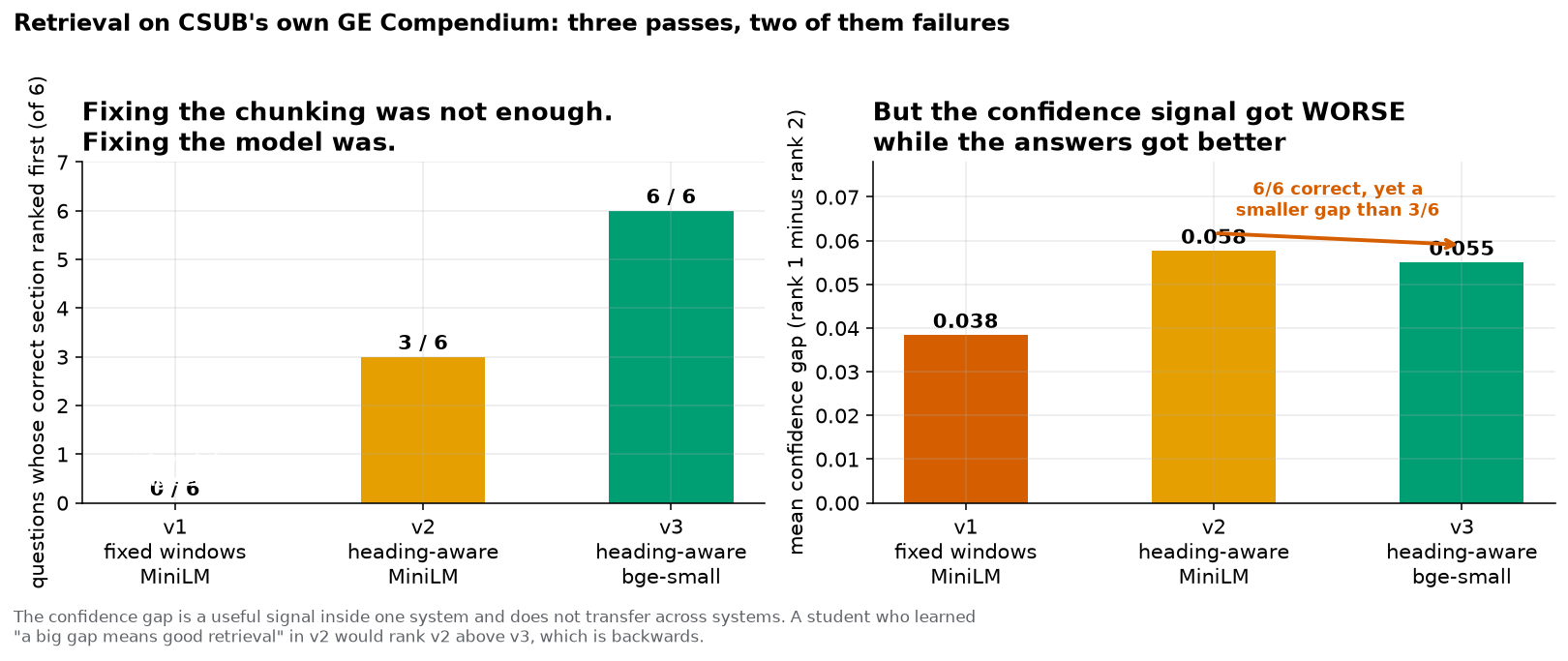
Two bar charts. The left chart counts questions whose correct section ranked first, out of — six: pass one is drawn at zero and labelled “0 / 6”, pass two reaches three, pass three reaches six. The right chart shows the mean confidence gap for the same three passes: 0.038, then 0.058, then 0.055, with an arrow marking that the third pass has a smaller gap than the second despite answering twice as many questions correctly. :width: 100%

The general form of the mistake

This chapter’s sting is a special case of something you will meet again in Chapter 13, where one model, one set of twenty questions and three different scoring procedures produce accuracies of 15.0%, 25.0% and 35.0% (real, from lab/out/we6b_eval_debiased.json).

The general statement is short. A number is a property of the procedure that produced it. Two numbers are comparable when they came out of the same procedure and are scored against something outside it. They are not comparable because they have the same name, the same units, or the same number of decimal places.

Questions worth asking whenever you meet two numbers side by side:

Did the same procedure produce both?
Is the thing they are scored against outside the procedure, or inside it?
If one system changed, how many things changed with it?

Common mistakes¶

These are the errors that actually happen, in the order you are most likely to make them.

Judging retrieval by the top score instead of the gap. A score of 0.910 means nothing on its own, because you do not know what the runner-up scored. In pass one the top score for the Area 2 question was 0.659, which sounds respectable, and it was the wrong section by a margin of 0.034 over the second-wrong section. Always look at rank 2.
Rounding before subtracting. Gaps are small differences between larger numbers, which is the situation where early rounding does the most damage. From the printed scores, $0.089 - 0.062 = 0.027$ ; from the full precision the machine holds, the answer is 0.028. Round once, at the end. See Toolkit Section 16.
Comparing a gap across two systems. This is the chapter’s central warning. Pass three beat pass two 6 to 3 while recording a smaller mean gap. Inside one system, a bigger gap means more confidence. Between two systems, a gap comparison is meaningless.
Believing that a bigger $k$ is safer. Sending more passages sends more tokens, spends more of the context length, costs more energy, and surrounds the answer with text that is not the answer. At $k = 6$ in the six-sentence run, 25 of the 37 words you send are off-topic.
Saying “the model was trained on our documents” when you mean retrieval. Retrieval changes the prompt. Training changes the parameters. They have different costs and different failure modes, and confusing them in writing will cost you marks in this course and credibility everywhere else.
Concluding “the embedding model is bad” from a failed retrieval. Pass one’s failure had nothing to do with the embedding model. The same model, given chunks that carried their headings, went from returning Area 6 text to answering 3 of 6. Check the chunking first; it is cheaper to fix and it is wrong more often.
Changing several things at once and then explaining the result. Pass one to pass two changed the corpus, the chunking and one question’s wording, so the rise from 0.038 to 0.058 cannot be credited to any one of them. Pass two to pass three changed exactly one thing, which is why its result can be believed.
Treating “3 of 6” as a precise measurement. With six questions, one question changing its answer moves the score by 16.7 percentage points. These are directions of travel. Chapter 12 shows how wide the honest interval around a number like this really is.
Forgetting the query prefix. bge-small-en-v1.5 expects "Represent this sentence for searching relevant passages: " on the front of the query and nowhere else. Leaving it off, or putting it on the passages too, gives a model that was asked to do a job it was not trained for.

What to remember¶

Retrieval turns the question and every passage into lists of numbers, scores each passage against the question with cosine similarity, and hands back the highest, which is nearest-neighbour search and nothing more. What tells you it worked is not the top score but the gap beneath it: in the measured six-sentence run, rank 2 scored 0.719 and rank 3 scored 0.089, and that drop of 0.630 is where the sentences about Kern County ran out. On a real document the method failed twice before it worked, first because fixed windows do not know which section they are in, then because a mislabelled chunk kept winning questions it did not answer. Fixing the chunking took the score to 3 of 6 and changing the embedding model took it to 6 of 6, with one variable moved and everything else held still. And the system that answered all six had a smaller mean gap than the one that answered half, which is the chapter’s real lesson: a diagnostic number belongs to the procedure that produced it and cannot be carried across to another one.

Lab 2 grows out of this chapter¶

Lab 2 points this exact pipeline at a Kern County or CSUB corpus of your choosing: the GE Compendium, a city or county document, a campus policy, a set of local news reports. You will write six questions with known answers, build the chunks, run the search, score it with Formula 10.7, and report the gaps with Formula 10.6.

Three things are graded, and only one of them is “did it work”.

Did you write the answer key before you ran the search? A retrieval result you score afterwards is not a measurement.
Can you diagnose your failures? Open the winning chunk, read it, and say why it won. The most valuable page in your report will be the one about a question the system got wrong.
Did you keep your comparisons honest? If you compare two setups, say how many variables moved between them.

Lab 2 is worth 100 points of the 1000 in this course and it reinforces quantitative reasoning and critical thinking. The rubric is in the syllabus.

Practice problems¶

Twenty-six problems in three tiers. Warm-up checks that you can do the arithmetic. Practice checks that you can apply it. Stretch checks that you can reason with it.

Worked solutions to the odd-numbered problems are in the answers appendix. Try each problem all the way to a number before you look.

Unless a problem says otherwise, round every final answer to three decimal places and keep full precision until the last step. See Toolkit Section 16 if rounding rules are hazy.

Every number in these problems is made up for practice unless it is marked real. Every number marked real names the file in lab/out/ that holds it, and you can open that file and check it.

Warm-up¶

1. Compute the dot product of $\mathbf{q} = (2, 6)$ and $\mathbf{d} = (3, 1)$ . Show both multiplications and the addition.

2. Using the two vectors from problem 1, compute $\lVert \mathbf{q} \rVert$ and $\lVert \mathbf{d} \rVert$ , then compute the cosine similarity $\cos(\mathbf{q}, \mathbf{d})$ with Formula 10.1. Write down every step.

3. Shrink $\mathbf{a} = (6, 8)$ to a unit vector by dividing each number by its length. Then check your answer by computing the dot product of the result with itself; it must come to 1.

4. A retrieval run returns four passages with cosine similarities, already sorted: 0.744, 0.701, 0.340, 0.298. Compute the confidence gap $g$ using Formula 10.4.

5. Using the same four scores, compute the drop at every possible cut, $g_1$ , $g_2$ and $g_3$ , using Formula 10.5. Say where you would cut, and give the number that justifies it.

6. Four questions produce confidence gaps of 0.120, 0.045, 0.061 and 0.018. Compute the mean gap $\bar{g}$ with Formula 10.6, adding the gaps two at a time so your working is visible.

7. A retrieval run is asked 9 questions and puts the correct section first on 4 of them. Compute hits@1 as a decimal and as a percentage, rounded to one decimal place.

8. One of these four numbers cannot be a cosine similarity: 0.93, -0.21, 1.40, 0.00. Say which, and say in one sentence how you know without computing anything.

9. A prompt is built from three retrieved passages of 48, 60 and 52 words. The 60-word passage turns out to be off-topic. What share of the words you sent is off-topic? Give your answer as a percentage to one decimal place.

10. all-MiniLM-L6-v2 has 22,713,216 parameters and bge-small-en-v1.5 has 33,360,000 (real, from lab/out/lab2_rag_v3.json). How many more parameters does the second have, and what is the ratio of the second to the first, to two decimal places?

Practice¶

11. A query embeds to $\mathbf{q} = (1, 0)$ and three passages embed to $\mathbf{d}_1 = (2, 0)$ , $\mathbf{d}_2 = (0, 5)$ and $\mathbf{d}_3 = (-3, 0)$ . Compute all three cosine similarities, name the nearest neighbour using Formula 10.3, and compute the confidence gap. Then say in one sentence what a cosine of -1 means about $\mathbf{d}_3$ .

12. In the measured six-sentence run the drops between neighbouring ranks were 0.191, 0.630, 0.028, 0.006 and 0.044 (real, from lab/out/we5_embeddings.json). You may send exactly two sentences to the model. Say which two, and justify the choice with one number from that list.

13. Explain to a classmate who has not read this chapter, in four sentences and using no symbols at all, why the Python code in Section 10.2 never divides by a length.

14. Pass one had a mean gap of 0.038 and a largest single gap of 0.076. The six-sentence run in Section 10.2 had a single gap of 0.191. Compute $0.191 \div 0.076$ and $0.191 \div 0.038$ , each to two decimal places, and write one sentence saying what the two answers tell you about how much harder the real corpus is.

15. A retrieval system returns five passages with scores 0.612, 0.609, 0.607, 0.601 and 0.598. Compute $g$ , compute all four drops, and compute the spread from the highest score to the lowest. Then say whether you would paste the rank-1 passage into a prompt, and why.

16. Your corpus has 248 chunks and every question you ask returns a rank 1. Explain, in three or four sentences, why “the system returned an answer” is not evidence that the answer is in the corpus. Use the word “gap” at least once.

17. Write down everything that changed between pass one and pass two, and everything that changed between pass two and pass three. Then say which of the two comparisons can support a claim of the form “X caused Y”, and why the other cannot.

18. A vendor writes: “Our retrieval system achieved 94% accuracy on our internal benchmark, while the leading competitor scores only 0.31 on their published confidence metric.” Give two separate reasons those two numbers cannot be compared. At least one of your reasons should use something measured in this chapter.

19. Pass two answered the Theme S question correctly at rank 1 with a gap of 0.004 (real, from lab/out/lab2_rag_v2.json). Suppose the rank-2 chunk’s score had been 0.005 higher. What would the new gap be, which chunk would be at rank 1, and would the question have been scored a hit? Write one sentence about how much you would rely on a result with a gap that size.

Stretch¶

20. Write a seventh question for the GE Compendium corpus, together with the heading of the section that answers it. Write the heading down before you would run any search. Then explain, in a short paragraph, why writing the answer down first changes what the run is capable of telling you.

21. Pass two’s semantic attractor was a chunk labelled Capstone Course Requirements that actually contained a prerequisite table, because the heading list in the code stops before the appendix. Propose two different fixes for this. For each one, say what it would cost in effort and what new way it could go wrong.

22. The mean gap does not transfer between embedding models. Propose a way of putting two systems’ gaps on a comparable footing. Then say what could still go wrong with your proposal, and whether hits@1 would still be the better number to report.

23. With $n = 6$ questions, one question changing its answer moves hits@1 by $1 \div 6 = 0.167$ , which is 16.7 percentage points. How many questions would you need before a single question moves the score by less than one percentage point? Show the inequality you solved and check your answer by computing $1 \div n$ for your value of $n$ . The signs $<$ and $>$ are unpacked in Toolkit Section 19.

24. In Chapter 13, one model answering one set of twenty questions produces accuracies of 15.0%, 25.0% and 35.0% under three different scoring procedures (real, from lab/out/we6b_eval_debiased.json). Write a short paragraph connecting that result to this chapter’s finding that a 6-of-6 system recorded a smaller mean gap than a 3-of-6 system. Name the single principle both results illustrate.

25. Retrieval adds tokens to the prompt. Chapter 7 measured Qwen2.5-0.5B-Instruct at 0.767 joules per token (real, from lab/out/theme_s_energy.json). A classmate proposes multiplying that number by the extra words to cost out sending four passages of 160 words instead of one. Give at least three reasons that calculation would not be sound. One of your reasons should be about what the 0.767 was measured on, and one should be about the difference between words and tokens.

26. Write one paragraph, at most 200 words, that you would hand to the CSUB advising office. It should say what a retrieval chatbot built over the GE Compendium can be trusted to do, what it cannot, and what a member of staff should check before believing an answer. Cite at least two numbers from this chapter, and name the file each one came from.

Where this goes next¶

Chapter 11 turns the question round. Instead of asking whether a model can find the right page, it asks whether a model can pass a test, and it runs into the same problem in a new form: a score means nothing until you know how it was produced and how much it would move if you asked a different set of questions.

The bridge between the two chapters is one sentence, and you have already met it twice. A number is a property of the procedure that produced it.