Chapter 9, Similarity is geometry.
This is a keystone chapter. Everything in Module D leans on the one idea in it, and Chapter 10 cannot be read without it. Take it slowly. Most people need two passes at Section 9.3, and that is what Section 9.3 is like.
What you need before this chapter
This is an honest list. If any line in it sounds unfamiliar, follow the link, read that section of the Math Toolkit, and come back. Nothing here is assumed.
| You need | Where it is taught from zero |
|---|---|
| A letter standing for a number, so that can mean “any number you like” | Math Toolkit, section 1: A letter standing for a number |
| What a pair of numbers like means, and how it becomes an arrow | Math Toolkit, section 14: Coordinates and vectors |
| The dot product: multiply matching numbers, add the products | Math Toolkit, Formula 15 |
| Square roots, and what means | Math Toolkit, section 9: Square roots |
| The length of an arrow, written with double bars | Math Toolkit, section 15: Absolute value and magnitude |
| Multiplication written four different ways, including two letters side by side | Math Toolkit, section 3 |
| The fraction bar as an instruction to divide | Math Toolkit, section 4 |
| , the symbol that says “add these up” | Math Toolkit, section 10: Sigma notation |
| The Greek letter , and how to say it | Math Toolkit, section 20: Greek letters |
| Rounding to four decimal places | Math Toolkit, section 16: Rounding |
| The signs and , and what “between -1 and 1” means | Math Toolkit, section 19: Inequality signs |
| Turning a decimal like 0.15 into a percentage | Math Toolkit, section 11: Percentages |
| Why a percentage point is not the same thing as a per cent | Math Toolkit, section 11, percentage points |
| What “3 out of 6” means as a number | Math Toolkit, section 12: Proportions |
| Reading a grid of numbers off a coloured chart | Math Toolkit, section 13: Reading a graph |
You do not need trigonometry. The word “cosine” comes from trigonometry, and this chapter uses none of it. You will meet the word as the name of a fraction you can compute with a phone calculator, and that is all it has to be here.
You do not need to have written code before. Every line of Python on this page is explained on the line it appears.
Setting up
Here is the whole chapter’s Python plumbing. It goes in one cell, at the top, and it is not repeated anywhere else on this page. That is a house rule in this course, borrowed from UC Berkeley’s Data Science Modules: every import lives in the first cell, one per line, each with a comment saying what it is for. Read the cell once and you know everything the rest of the page depends on.
# Cell 1. Every import this chapter uses. Run this once, at the top, before any other cell.

import os                                              # lets Python read and change settings on your computer
os.environ["HF_HOME"] = r"C:\math3219\models"          # where downloaded models are kept; MUST come before the model import below

import math                                            # square roots, and the arccos that turns a cosine back into an angle
from sentence_transformers import SentenceTransformer  # turns a whole sentence into one list of 384 numbers
Four lines do four separate jobs.
import os gives Python a way to talk to the machine it is running on. The next line uses it
to say where model files should live, and it has to come before the model library loads,
because that library reads the setting the moment it starts. The r in front of the quotation
marks tells Python to take the backslashes literally instead of treating them as instructions.
import math brings in square roots and the inverse cosine. Both appear later on this page.
from sentence_transformers import SentenceTransformer reaches into a library and pulls out
one named piece. That piece is what turns a sentence into a list of numbers. Section 9.5
compares six sentences of 384 numbers each, and six lots of 384 is
numbers in total. This library handles the loading and the arithmetic for all of them.
If any of those lines produces a red error message, go to the Python reference on installing the tools. Nothing in this chapter is graded on getting the install right on the first try.
Two sentences about a city, and a number
Here are two sentences about the place this university sits in.
Bakersfield is in Kern County, California.
Kern County’s largest city is Bakersfield.
A person reads those and sees the same fact twice, written from two directions. A computer reads two strings of characters. Getting from the second reading to the first is the whole problem, and this chapter is where the course solves it.
Now here is the pair that shows why the obvious approach fails.
The cat sat on the mat.
A kitten rested on the rug.
Anyone reading those two lines pictures nearly the same scene. Now count the words they share. “The”, “on”, and “a”. Every word that carries the meaning is different. Cat is not kitten. Sat is not rested. Mat is not rug. A program that compares two sentences by counting shared words, which is how search worked for decades, scores that pair at close to nothing. It would rank a sentence about “the cat sat on the chair” far above it, because two of the important words match.
A small model on the course machine scored the cat sentence and the kitten sentence at
0.6124, on a scale where 1 is the highest possible. It scored the two Bakersfield sentences
at 0.8333, the highest pair in the whole run. Both numbers are real, from
lab/out/we5_embeddings.json.
So the question is: where does a number like 0.8333 come from?
Chapter 8 did the first half. It turned a sentence into a vector, which is a list of numbers you can also picture as an arrow. This chapter does the second half. It takes two arrows and produces one number saying how alike they are.
And the first honest attempt at that number is wrong, in a way that is worth seeing, because the fix for it is the entire chapter. Here is the fix in one line, and it is the line to remember:
The arrow and the arrow have a cosine similarity of exactly 1.0000, because the second arrow is the first one doubled. Same direction, twice the length. Length is not meaning. Direction is.
That single line is why every similarity formula in every search engine and every retrieval system divides by the lengths. It is not a ritual. It is a repair.
Learning objectives
By the end of this chapter you will be able to:
Compute the dot product and the length of a vector by hand, writing out every multiplication and every addition.
Compute the cosine similarity of two vectors by hand, and state what its value means on the scale from -1 to 1.
Explain why cosine similarity divides by both lengths, using the pair and as the evidence.
Read a similarity matrix produced from real sentence embeddings, including its diagonal, its symmetry, and its negative entries.
Design a comparison in which one variable is changed and everything else is held fixed, and say what goes wrong in a comparison where two things change at once.
Durable skills practised in this chapter: quantitative reasoning, through hand computation and the interpretation of a measured similarity; and critical thinking, through the experimental-control section, where you judge whether a comparison can support the conclusion drawn from it.
This lesson at a glance
The dot product measures two things at the same time, direction and length, and for comparing meaning only one of them is wanted.
Cosine similarity is the dot product divided by both lengths, which removes length and leaves direction, on a fixed scale from -1 to 1.
A vector and the same vector doubled score exactly 1.0000, which is the proof that the division is doing real work rather than tidying.
A comparison is only worth something when one variable moves and everything else is held still, which is the standard this course holds every later measurement to.
The vocabulary of this chapter
Every technical word on this page is in this table, defined before it is used. Read it once now. Come back to it whenever a word stops making sense. No word in the right-hand column is defined using a word you have not already met.
| Word | What it means, in one line |
|---|---|
| origin | The point , where the two axes of a graph cross. Every arrow in this chapter starts there. |
| vector | An ordered list of numbers, which you can also picture as an arrow drawn from the origin. |
| coordinate | One of the numbers in a vector. has two coordinates, 3 and 4. |
| dimension | How many numbers a vector holds. has dimension 2. A sentence vector here has dimension 384. |
| dot product | Multiply the matching coordinates of two vectors, then add up all the products. One number comes out. |
| length | How long the arrow is. Also called the magnitude or the norm. Written with double bars. |
| scalar | A single ordinary number, as opposed to a whole vector. The 2 in “double it” is a scalar. |
| scaling | Multiplying every coordinate of a vector by the same scalar, which stretches or shrinks the arrow. |
| cosine similarity | The dot product of two vectors divided by both of their lengths. A number from -1 to 1. |
| degree | The unit turning is measured in. A full turn is 360 degrees, a square corner is 90 degrees. |
| radian | A second unit for the same job. A full turn is about 6.283185 radians instead of 360 degrees. Python works in radians and this book reports degrees. |
| angle | How far apart two arrows point, measured in degrees. 0 degrees is the same direction, 180 degrees is opposite. |
| arccos | The undo button for cosine. Hand it a cosine and it hands back the angle. Written or . |
| orthogonal | At a right angle, meaning 90 degrees apart. The everyday word is perpendicular. |
| unit vector | A vector whose length is exactly 1. Its direction is kept and its length is thrown away. |
| normalising | Dividing every coordinate of a vector by that vector’s length, which turns it into a unit vector. |
| embedding | A list of numbers that stands for a piece of text, arranged so that similar meanings give similar lists. |
| matrix | A rectangle of numbers, arranged in rows and columns. |
| transpose | The same matrix with its rows and its columns swapped over. Written with a raised capital T. |
| similarity matrix | A matrix holding the similarity of every item against every other item. |
| diagonal | The entries of a matrix running from the top left to the bottom right, where an item meets itself. |
| symmetric | A matrix that reads the same across the diagonal, so the entry in row 2 column 3 equals the one in row 3 column 2. |
| variable | Anything in an experiment that could take a different value. Size, model, wording, scoring rule. |
| held fixed | Kept identical across every condition of an experiment on purpose, so it cannot explain the result. |
| controlled experiment | A comparison in which exactly one variable is allowed to change and every other variable is held fixed. |
| confounded | When two variables change together, so you cannot tell which one caused the result. |
| manipulation check | A quick sum run before you trust a result, confirming that the variables you meant to hold fixed really did stay fixed. |
| corpus | A collection of documents a system searches through. This course uses real CSUB and Kern County documents. |
| standard error | A measure of how far a score would be expected to wander if you ran the same test on a fresh set of questions. Chapter 12 builds it from zero. |
9.1 The dot product measures two things at once, and one of them is in the way
Intuition
Picture two people arguing about which route to take out of town. Both point. If their arms point the same way, they agree. If one points north and the other points east, they disagree. If one points north and the other points south, they disagree as hard as it is possible to disagree.
Now suppose one of them has a longer arm.
The direction they point is the opinion. The length of the arm is nothing at all. It is an accident of the person, not a fact about the route. Any measurement that lets arm length change the answer is measuring the wrong thing.
That is exactly the position the dot product puts you in.
Chapter 8 built the dot product. You take two vectors, multiply the matching numbers, and add up the products. The result is a single number that is large and positive when the two arrows lean the same way, near zero when they are at a square corner, and negative when they lean opposite ways. That behaviour is genuinely useful and it is why the dot product is the starting point.
The trouble is that the dot product also gets larger when either arrow gets longer, and it does that whether or not the directions changed at all. Two effects are stirred into one number, and from the number alone you cannot tell which effect produced it. A dot product of 50 might mean “these two point in very similar directions” or it might mean “these two are enormous”.
For sentences that is a real problem and not a theoretical one. Embedding models can hand back vectors of different lengths for different pieces of text. If length counts, then a long document can beat a short one on similarity without being any more relevant, and a search engine built on a raw dot product will quietly prefer whichever passage happens to have the bigger numbers in it.
So the plan for this section is to build the dot product carefully, build the length carefully, and then break the dot product on purpose, using a pair of arrows where the answer it gives is visibly absurd. Section 9.2 repairs it.
The mathematics
Two formulas are needed before the repair can be stated. Both appear here with every symbol defined, including the ones that look too ordinary to define.
Formula 9.1: the dot product
1. In words. Line the two lists of numbers up side by side. Multiply the first number of one list by the first number of the other. Multiply the second by the second. Keep going to the end of the lists. Add all of those products together. The total is the dot product.
2. The formula. For two vectors that each hold numbers:
Written out for two numbers each, with nothing hidden:
3. The symbols.
| Symbol | How to say it out loud | What it means |
|---|---|---|
| “vector a”, or “bold a” | a whole vector, printed in bold. The bold type is the signal that this is a list of numbers rather than one number. | |
| “vector b” | the other vector. It must hold the same count of numbers as . | |
| “dot” | the dot product. Between two bold letters this raised dot means this whole operation. It is not ordinary multiplication. | |
| “equals” | the thing on the left and the thing on the right are the same number. | |
| “sum”, or “sigma” | add up everything that follows, once for each value of the counter. See Math Toolkit section 10. | |
| “eye” | a counter. It takes the value 1, then 2, and so on. It is not a number in the data; it is a position number. | |
| underneath the | “i equals one” | start the counter at 1, meaning the first position. |
| above the | “capital dee” | stop the counter here. is how many numbers each vector holds. |
| “a sub i” | the number sitting in position of vector . See Math Toolkit section 2. | |
| “b sub i” | the number sitting in position of vector . | |
| “a sub i times b sub i” | multiply them. Two symbols written next to each other with nothing between them means multiply. See Math Toolkit section 3. | |
| , | “a sub one”, “a sub two” | the first and second numbers in . |
| “plus” | add. | |
| “times” | multiply. It appears in the worked example below rather than in the formula, because this book writes when the two things are plain numbers and writes when they are letters. Both mean multiply. See Math Toolkit section 3. |
4. Out loud. “a dot b is the sum, over every position, of a’s number at that position times b’s number at that position.”
5. Worked, with every step. Take and , so . These are not made up; they are the lab’s recorded pair.
Step 1, multiply the two first numbers.
Step 2, multiply the two second numbers.
Step 3, add the two products.
The same three steps are laid out again with more commentary in Worked Example 9.1, immediately below.
6. Check it. The answer must be one single number. If you finished holding a list, you forgot to add the products up. A second check: the dot product of a vector with itself can never be negative, because every term is a number multiplied by itself. If yours came out negative, you compared the wrong pair or dropped a minus sign.
Now the second formula, the one that measures how long an arrow is.
Formula 9.2: the length of a vector
1. In words. Square every number in the list, meaning multiply each one by itself. Add up all those squares. Take the square root of the total. The answer is the length of the arrow.
2. The formula. For a vector of two numbers:
For a vector of numbers:
3. The symbols.
| Symbol | How to say it out loud | What it means |
|---|---|---|
| “the length of a”, or “the norm of a” | the answer: how long the arrow is. | |
| the double upright bars | “the length of” | they are the instruction. Single bars around a plain number mean something different, the absolute value; see Math Toolkit section 15. |
| “equals” | the thing on the left and the thing on the right are the same number. | |
| “the square root of” | the number which, multiplied by itself, gives what is underneath. because . See Math Toolkit section 9. | |
| the bar across the top of the root sign | no sound | it shows how far the square root reaches. Everything under the bar is inside the root. |
| “a sub one squared” | the first number multiplied by itself. | |
| the raised 2 | “squared” | multiply the thing by itself once. See Math Toolkit section 5. |
| “plus” | add. | |
| “the sum from i equals one to capital dee” | add up one square for each position in the list. |
4. Out loud. “The length of a is the square root of the sum of the squares of its numbers.”
5. Worked, with every step. Find the length of .
Step 1, square each coordinate.
Step 2, add the squares.
Step 3, take the square root.
Worked Example 9.2, immediately below, does this again for a second vector, and that second one is the one this chapter turns on.
6. Check it. A length is never negative, because squaring destroys every minus sign. A length is zero only when every coordinate is zero. And a length is always at least as big as the largest single coordinate, ignoring its sign: for the length must come out at 4 or more, and it comes out at 5. If yours came out smaller than the biggest coordinate, you forgot to square something.
Now break it on purpose
Here is the demonstration that the dot product on its own cannot be the answer.
Compare with itself. Nothing could be more similar to than .
Now compare with , which is a different arrow.
Read those two lines next to each other.
| Comparison | Dot product |
|---|---|
| against itself | 25 |
| against | 50 |
If you rank by raw dot product, is twice as similar to as it is to itself. That is not a subtle bias. It is nonsense, and the arithmetic producing it is completely correct. The formula is doing what it was built to do. It was built to do the wrong job.
Python
The first cell builds the dot product of and one multiplication at a time, so that nothing is hidden inside a library call. There is a one-line way to do this in numpy. It is not used here, because the point of this cell is to watch the arithmetic happen.
# Cell 2. The dot product of two vectors, written as a loop so every step is visible.

first_vector = [3, 4]        # the arrow this chapter calls a
second_vector = [6, 8]       # the arrow this chapter calls d, which is a doubled

dot_product = 0              # the running total starts at zero, before anything has been added

for coordinate_position in range(2):                                            # takes the value 0, then the value 1
    one_product = first_vector[coordinate_position] * second_vector[coordinate_position]   # multiply the matching pair
    print("position", coordinate_position, ":", first_vector[coordinate_position], "times", second_vector[coordinate_position], "=", one_product)
    dot_product = dot_product + one_product                                     # add that product to the running total

print("dot product of a and d:", dot_product)
Output:
position 0 : 3 times 6 = 18
position 1 : 4 times 8 = 32
dot product of a and d: 50
Six things in that cell are worth naming, because they come back on every later page.
first_vector = [3, 4] makes a list: several values in order, inside square brackets,
separated by a comma. A list is how Python holds a vector.
dot_product = 0 sets a running total before the loop starts. Every addition afterwards
adds onto this. Starting at 0 matters, because 0 is the number that changes nothing when you
add it.
for coordinate_position in range(2): is a loop. range(2) produces the positions 0 and
1, and the indented lines underneath run once for each. Python counts from 0, so position 0
is the first coordinate and position 1 is the second. That trips up nearly everybody once.
first_vector[coordinate_position] reads “the item of first_vector at this position”. On the
first pass it is 3, on the second it is 4.
dot_product = dot_product + one_product looks strange as a piece of English, because it looks
like it says a thing equals itself plus something. It does not. The single equals sign in Python
means “work out the right-hand side, then store it under the name on the left.” So it means
“take the total you have, add the new product, and let that be the new total.”
The printed line inside the loop is there only so you can see the multiplications. It matches Steps 2 and 3 of Worked Example 9.1 exactly, and the final total matches Step 4.
Now the lengths, and then the comparison that breaks.
# Cell 3. The length of each vector, and the comparison that shows the dot product is not enough.

sum_of_squares_first = 0                                   # running total of squared coordinates for a
for coordinate_position in range(2):
    sum_of_squares_first = sum_of_squares_first + first_vector[coordinate_position] * first_vector[coordinate_position]
length_first = math.sqrt(sum_of_squares_first)             # square root of the total gives the length

sum_of_squares_second = 0                                  # the same three lines again, for d
for coordinate_position in range(2):
    sum_of_squares_second = sum_of_squares_second + second_vector[coordinate_position] * second_vector[coordinate_position]
length_second = math.sqrt(sum_of_squares_second)

print("sum of squares for a:", sum_of_squares_first, " length of a:", length_first)
print("sum of squares for d:", sum_of_squares_second, " length of d:", length_second)

dot_with_itself = 0                                        # now compare a against a copy of itself
for coordinate_position in range(2):
    dot_with_itself = dot_with_itself + first_vector[coordinate_position] * first_vector[coordinate_position]

print("a compared with itself, dot product only:", dot_with_itself)
print("a compared with d,      dot product only:", dot_product)
Output:
sum of squares for a: 25  length of a: 5.0
sum of squares for d: 100  length of d: 10.0
a compared with itself, dot product only: 25
a compared with d,      dot product only: 50
The length code is written out twice on purpose, once for each vector, rather than folded into something reusable. Repetition is easier to read when you are learning, and this course chooses readable over clever every time.
math.sqrt is the square root. It comes from the math library imported in Cell 1, which is
why the name has math. in front of it.
5.0 is printed rather than 5 because math.sqrt always hands back a number with a decimal
point, whether or not the answer is whole. The value is 5 exactly.
The last two lines are the failure, printed. 25 against 50. The arrow is ranked as twice as similar to a different arrow as it is to itself, and every multiplication that produced those numbers is correct.
9.2 Cosine similarity: divide the length out
Intuition
Two students take two different tests. One scores 18. The other scores 45. Who did better?
You cannot say, and not because the question is hard. The question is incomplete. Eighteen out of what? Forty-five out of what? Once you learn that the first test was out of 20 and the second was out of 60, the comparison becomes easy: and . The first student did better, even though their raw score was smaller. All four of those numbers are made up for practice, and they are small enough to check on a phone.
The sign in those two lines is the division sign, said “divided by”. It does the same job as a fraction bar: and are two ways of writing the same instruction. This chapter uses when the division happens on one line and a fraction bar when the top and the bottom each need room of their own. See Math Toolkit section 4.
Dividing by the total is what made the two scores comparable. It put both onto the same fixed scale, from 0 to 1, where the size of the original test no longer counts for anything. Nobody finds that step mysterious. Everybody has done it since primary school.
Cosine similarity is that same step, done for arrows.
The dot product is the raw score. The two lengths are the two different totals. Divide the raw score by both lengths and you get a number on a fixed scale, from -1 to 1, on which the sizes of the two original arrows no longer count for anything. What is left is direction alone, which is exactly the part that carries the meaning.
The name is borrowed from trigonometry. In trigonometry, the cosine of an angle is a number between -1 and 1 that tells you how far the angle is from pointing straight ahead. It turns out that this fraction, dot product over the two lengths, gives exactly the cosine of the angle between the two arrows, which is where the name comes from. You do not need any trigonometry to use it. If you can divide, you can compute a cosine similarity. The trigonometry is a bonus explanation, not a prerequisite.
One warning that belongs here rather than later. Cosine similarity is not a distance. A distance is small when two things are alike and grows as they move apart. Cosine does the opposite: it is largest, at 1, when two things point the same way, and it falls toward -1 as they move apart. Reading a cosine as a distance reverses every conclusion you draw from it.
The mathematics
Formula 9.3: cosine similarity
1. In words. Work out the dot product of the two vectors. Work out the length of each one. Multiply the two lengths together. Divide the dot product by that product. The answer is the cosine similarity.
2. The formula.
Written out with nothing hidden, for two vectors of numbers each:
That second version looks worse and says exactly the same thing. It is the first version with Formula 9.1 poured into the top and Formula 9.2 poured into the bottom, twice. Nothing new has been introduced.
3. The symbols.
| Symbol | How to say it out loud | What it means |
|---|---|---|
| “cosine of a and b” | the answer: a number from -1 to 1. | |
| the round brackets and the comma | “of ... and ...” | they hold the two vectors the answer depends on. They do not mean multiply. |
| “equals” | the two sides are the same number. | |
| “a dot b” | the dot product, Formula 9.1. This is the top of the fraction. | |
| the fraction bar | “divided by” | divide the whole top by the whole bottom. The bar has invisible brackets around each half; see Math Toolkit section 4. |
| “divided by” | the same instruction as the fraction bar, written on one line. and mean the identical thing. | |
| “the length of a” | the length, Formula 9.2. | |
| “the length of b” | the length of the other vector. | |
| the small gap between the two lengths | “times” | multiply the two lengths together. A gap between two symbols means multiply. |
| “the sum from i equals one to capital dee” | add up one term per position. | |
| “the square root of” | as in Formula 9.2. | |
| , | “a sub i”, “b sub i” | the numbers at position in each vector. |
| -1 | “minus one” | the smallest value a cosine similarity can take. “Between -1 and 1” includes both ends; see Math Toolkit section 19. |
4. Out loud. “The cosine similarity of a and b is their dot product, divided by the length of a times the length of b.”
Say that sentence out loud once before reading on. It is three nouns and two operations, and once you can say it you can rebuild the formula from memory.
5. Worked, with every step. Take and .
Step 1, the dot product, using Formula 9.1.
Step 2, the length of , using Formula 9.2.
Step 3, the length of .
Step 4, multiply the two lengths.
Step 5, divide the dot product by that product.
Worked Example 9.3, below, walks the same five steps with more commentary, and Worked Example 9.4 does a second pair whose answer comes out at zero.
6. Check it. The answer must land between -1 and 1. If it did not, something went wrong, and the most common cause by a wide margin is forgetting a square root, which makes the bottom of the fraction far too small. The second most common cause is dividing by one length instead of two. A second check you can always run: the cosine similarity of any vector with itself must be exactly 1. Try it on your own vector, and if it does not come out at 1, the mistake is in your arithmetic and not in the formula.
Python
This cell computes cosine similarity for three different partners of the same vector . The three partners are , , and . Every one of those three answers is in the lab’s recorded file, so you can check the code against a number nobody typed by hand.
# Cell 4. Cosine similarity for three partners of the same vector, computed from scratch.

vector_a = [3, 4]                                  # the vector every comparison is made against
partner_vectors = [[4, 3], [-4, 3], [6, 8]]        # a list holding three vectors: b, then c, then d
partner_names = ["b", "c", "d"]                    # the names used for them in the text above

for partner_position in range(3):                  # takes the value 0, then 1, then 2
    one_partner = partner_vectors[partner_position]        # pull out one of the three vectors
    running_dot = 0                                        # running total for the dot product
    squares_of_a = 0                                       # running total of a's squared coordinates
    squares_of_partner = 0                                 # running total of the partner's squared coordinates
    for coordinate_position in range(2):                   # walk along the two coordinates
        running_dot = running_dot + vector_a[coordinate_position] * one_partner[coordinate_position]
        squares_of_a = squares_of_a + vector_a[coordinate_position] ** 2
        squares_of_partner = squares_of_partner + one_partner[coordinate_position] ** 2
    length_of_a = math.sqrt(squares_of_a)                  # Formula 9.2, for a
    length_of_partner = math.sqrt(squares_of_partner)      # Formula 9.2, for the partner
    cosine_value = running_dot / (length_of_a * length_of_partner)   # Formula 9.3
    print(partner_names[partner_position], one_partner,
          " dot =", running_dot,
          " lengths =", round(length_of_a, 4), "and", round(length_of_partner, 4),
          " cosine =", round(cosine_value, 4))
Output:
b [4, 3]  dot = 24  lengths = 5.0 and 5.0  cosine = 0.96
c [-4, 3]  dot = 0  lengths = 5.0 and 5.0  cosine = 0.0
d [6, 8]  dot = 50  lengths = 5.0 and 10.0  cosine = 1.0
Three rows, and every number in them was computed by hand earlier on this page.
Row b: dot 24, lengths 5 and 5, cosine 0.96. That is Worked Example 9.3.
Row c: dot 0, lengths 5 and 5, cosine 0.0. That is Worked Example 9.4.
Row d: dot 50, lengths 5 and 10, cosine 1.0. That is the next section, and it is the reason
this chapter exists.
Five pieces of the code deserve a name.
partner_vectors = [[4, 3], [-4, 3], [6, 8]] is a list of lists. The outer square brackets
hold three items, and each item is itself a list of two numbers. partner_vectors[0] is the
whole list [4, 3].
** is Python’s way of writing “raised to the power of”, so vector_a[coordinate_position] ** 2
is that coordinate squared. It does the same job as multiplying the coordinate by itself, and it
is written this way here because it reads closer to the in Formula 9.2.
There is a loop inside a loop. The outer loop picks one partner vector. The inner loop walks along that partner’s two coordinates. The inner loop finishes all its work before the outer loop moves to the next partner. That structure is worth recognising, because Section 9.5 uses the same shape to fill a whole table.
The three running totals are reset to 0 at the top of every pass of the outer loop. If they were not, the second partner would inherit the first partner’s totals and every answer after the first would be wrong. That is one of the most common bugs in code of this shape.
round(cosine_value, 4) rounds to four decimal places. Notice what Python prints: 0.96, not
0.9600, and 1.0, not 1.0000. Python drops trailing zeros when it prints a number. The value
is identical; only the printing is shorter. This book writes 0.9600 and 1.0000 in prose because
four decimal places is the chapter’s stated precision, and Python writes 0.96 and 1.0 because
that is Python’s habit. Neither one is more accurate than the other.
9.3 The keystone: doubling an arrow changes nothing
Intuition
This is the section the chapter is named for. Read it twice.
Draw an arrow from the origin to the point . Now draw a second arrow from the origin to the point . Look at what the second arrow is. Six is two times three. Eight is two times four. Every coordinate has been doubled, and doubling every coordinate stretches the arrow without turning it at all. The second arrow lies exactly on top of the first one and carries on past its tip. Same line. Same direction. Twice the length.
Now ask the question that matters. Are those two arrows pointing the same way?
They are, and there is no room to argue about it, because the second arrow is drawn along the first one. If the direction is the meaning, then those two arrows mean the identical thing. A measurement of similarity that does not return its top score for that pair is broken.
The raw dot product returns 50 for that pair, and 25 when is compared with itself. It is broken.
Cosine similarity returns exactly 1.0000, and the angle between the two arrows is exactly 0.00 degrees. Not close to 1. Not 1 after rounding. Exactly 1, and the arithmetic in the next part shows that it could not have come out as anything else.
That is the moment dividing by the lengths stops being a step you copy and becomes a step you understand. The division is not there to make the numbers tidy. It is there to delete a variable, length, that was contaminating the answer, so that the only thing left in the number is the variable you actually wanted, direction.
Why does any of this matter for sentences? Because an embedding model can give you back vectors of different lengths for two pieces of text that mean the same thing. The length can depend on how long the text is, or on quirks of the model, or on nothing you can name. If length counts, those accidents count. The cosine says: whatever the lengths are, throw them away, and tell me only whether these two point the same way.
The mathematics
First, the operation that made out of needs a name.
Formula 9.4: scaling a vector, and what it does to length and to cosine
1. In words. If you multiply every number in a vector by the same positive number, the arrow keeps pointing exactly where it pointed and its length is multiplied by that same number. Because of that, the cosine similarity between the original vector and the scaled one comes out at exactly 1, no matter what positive number you used.
2. The formula. Write for the vector you get by multiplying every coordinate of by the scalar . Then, for any greater than 0:
3. The symbols.
| Symbol | How to say it out loud | What it means |
|---|---|---|
| “kay” | the scalar you multiply by. A single ordinary number, such as 2 or 3 or 0.5. | |
| “k a”, or “k times vector a” | the new vector made by multiplying every coordinate of by . A scalar next to a bold letter means scale it. | |
| “the length of k a” | how long the stretched arrow is. | |
| “k times the length of a” | the scalar multiplied by the original length. The gap means multiply. | |
| “a dot a” | the dot product of with itself, which equals squared. | |
| “k times, bracket, a dot a” | a number written next to a bracket means multiply it by whatever the bracket holds. The brackets are there to say “work out the dot product first, then multiply by ”. They do not square anything and they do not mean anything else. See Math Toolkit section 3. | |
| the raised dot on the bottom of the middle fraction | “times” | a second job for the same mark. Between two bold letters, as in , the raised dot means the dot product of Formula 9.1. Between two ordinary numbers, as in , it means plain multiplication and nothing more. Lengths are ordinary numbers, so the dots on the bottom of that fraction are plain multiplication. See Math Toolkit section 3, which lists as one of the four ways to write . |
| “k is greater than zero” | must be positive for this to give 1. The sign opens toward the bigger side, so it says is on the bigger side of zero. See Math Toolkit section 19. A negative gives -1; see the note below. | |
| the three fractions joined by | “which equals ... which equals ...” | each fraction is the one before it, rewritten. Nothing new enters from left to right. |
| no sound; say “checks out” | a tick. It is not part of the arithmetic. It marks a line where a number you computed matched a number you predicted. |
4. Out loud. “The length of a scaled vector is the scalar times the original length, and so the cosine similarity of a vector with any positive multiple of itself is one.”
5. Worked, with every step. Take and , so .
Step 1, check the first line of the formula. The length of is 5, so the formula predicts the stretched arrow has length . Compute it directly to confirm:
Step 2, the dot product on the top of the cosine fraction.
Step 3, the product of the two lengths on the bottom.
Step 4, divide.
The top and the bottom are the same number, 50, which is why the answer is exactly 1. Worked Example 9.5, below, is the same arithmetic with more commentary, and the general argument for every positive follows it.
6. Check it. Scale any vector you like by any positive number you like, compute the cosine with the original, and you must get 1.0000 every time. If you get anything else, the arithmetic slipped. If you scale by a negative number, you must get exactly -1.0000, because the arrow now points the opposite way along the same line.
The same argument without particular numbers
Here is why it works for every positive , and not only for . Follow it slowly. This is four short steps and each one uses a rule from the Math Toolkit.
One thing changes from here on, and it is worth naming before it happens. Up to now every letter stood for something you could see: was and was 2. From here on , and stand for any numbers at all. That is the only reason to use letters: one argument written with letters covers every choice of numbers at once, so you do not have to run the arithmetic again for and again for and again forever. If a letter standing for an unknown number is the part that feels slippery, Math Toolkit section 1 starts that idea from nothing. You can also read every line below with , and in your head, and each line will come out to a number you have already seen on this page.
Three pieces of notation are about to be used, so here they are first, each one checked on small numbers you can verify on a phone. Nothing below this box is used before it appears here.
Step 1. The top of the fraction. The dot product of with is
Read that in three hops. The first hop is Formula 9.1 applied to and , whose coordinates are and . The second hop rewrites as , which is move One followed by move Three of the box above. The third hop is move Two: every term picked up a factor of , so a single can be taken out in front of the bracket.
Step 2. The length of the scaled vector.
Four hops this time. The first is Formula 9.2 applied to the vector whose coordinates are and . The second is move Three: becomes . The third is move Two, with as the shared multiplier this time instead of .
The fourth hop is the only new rule on this page, and it is worth a line of its own. A square root of two things multiplied together is the same as the two square roots multiplied together. In symbols, whenever neither nor is negative. So is times , and is , because multiplied by itself is . That last step is the one that needs to be positive: is the size of with any minus sign stripped off, so for a negative it would come back positive rather than as itself. Check the whole hop with and : , and . Same answer.
Step 3. The bottom of the fraction.
The raised dot in the middle is plain multiplication, not a dot product, because both sides of it are ordinary numbers rather than vectors. The step itself is this: a square root multiplied by itself gives back what was under the root, since that is exactly what a square root is. Here appears twice, once from each length, and the two of them collapse to , leaving the in front. Check it with and : , and . Same answer.
Step 4. Divide the top by the bottom.
The top and the bottom are the identical expression. Any number divided by itself is 1, as long as it is not zero, and it is not zero here as long as is not the zero vector.
Read what that says. The letter appears in the top and in the bottom and cancels. That cancellation is the removal of length from the answer. Everything about how long the arrows are went into , and went away.
Python
The cell below scales by five different amounts and computes the cosine similarity each time. The multiplier 2 is the lab-recorded case. The other four multipliers, 1, 3, 10 and 100, are made up for practice, to show that nothing special was happening at 2.
# Cell 5. Stretch the same vector by five different amounts and watch the cosine refuse to move.

multipliers = [1, 2, 3, 10, 100]                   # the five scalars, called k in Formula 9.4

for multiplier_position in range(5):                                  # 0, 1, 2, 3, then 4
    one_multiplier = multipliers[multiplier_position]                 # pull out one value of k
    stretched_vector = [vector_a[0] * one_multiplier, vector_a[1] * one_multiplier]   # multiply both coordinates by k
    running_dot = 0                                                   # reset all three totals for this value of k
    squares_of_a = 0
    squares_of_stretched = 0
    for coordinate_position in range(2):
        running_dot = running_dot + vector_a[coordinate_position] * stretched_vector[coordinate_position]
        squares_of_a = squares_of_a + vector_a[coordinate_position] ** 2
        squares_of_stretched = squares_of_stretched + stretched_vector[coordinate_position] ** 2
    length_of_a = math.sqrt(squares_of_a)
    length_of_stretched = math.sqrt(squares_of_stretched)
    cosine_value = running_dot / (length_of_a * length_of_stretched)
    print("k =", one_multiplier,
          " stretched vector =", stretched_vector,
          " dot =", running_dot,
          " length =", round(length_of_stretched, 4),
          " cosine =", round(cosine_value, 4))
Output:
k = 1  stretched vector = [3, 4]  dot = 25  length = 5.0  cosine = 1.0
k = 2  stretched vector = [6, 8]  dot = 50  length = 10.0  cosine = 1.0
k = 3  stretched vector = [9, 12]  dot = 75  length = 15.0  cosine = 1.0
k = 10  stretched vector = [30, 40]  dot = 250  length = 50.0  cosine = 1.0
k = 100  stretched vector = [300, 400]  dot = 2500  length = 500.0  cosine = 1.0
Read that output column by column, because the columns are the argument.
The dot column runs 25, 50, 75, 250, 2500. It grows by a factor of 100 from the first row to the last. The raw dot product is wildly sensitive to length.
The length column runs 5.0, 10.0, 15.0, 50.0, 500.0. Also a factor of 100 from top to bottom. This column is the manipulation working: each length is exactly times 5, which is Formula 9.4’s first line printed as data.
The cosine column runs 1.0, 1.0, 1.0, 1.0, 1.0. It does not move at all.
Two columns moved by a factor of 100 and the third did not move by anything. That is the division doing its job, and it is the single most important output in this chapter.
One line of code is worth naming.
stretched_vector = [vector_a[0] * one_multiplier, vector_a[1] * one_multiplier] builds a new
two-item list by multiplying each coordinate separately. It is written out coordinate by
coordinate rather than as a shortcut, because that is what scaling means and this is the cell
where scaling is being taught.
Three more details in that output repay a second look.
The first row uses , which changes nothing at all. Multiplying every coordinate by 1 gives back the same vector, so that row is compared with itself. Its cosine is 1.0, which is the sanity check from Formula 9.3 printed as data: any vector compared with itself must score 1. Putting a do-nothing row at the top of a table is a habit worth copying, because if the row that should change nothing does change something, the code is wrong and you have found out early.
The dot product column and the length column happen to grow at the same rate here, and that is a coincidence of this particular experiment. From to , the length goes from 5.0 to 500.0. Divide to see the factor: , so the length is 100 times bigger. The dot product goes from 25 to 2500, and , so it is also 100 times bigger. The two rates match here only because one of the two vectors is being stretched and the other is being left alone. Stretch both and the dot product would grow by , while each length grew by 100, so the two lengths multiplied together would also grow by . The cosine would still not move, because the bottom of the fraction grew exactly as fast as the top. That is Formula 9.4 with a on each side.
Nothing in the cosine column is rounded into looking right. round(cosine_value, 4) would
happily print 1.0 for a value of 0.99996. The reason every row reads 1.0 is that every row is 1,
and Worked Example 9.7 in Section 9.5 shows the same result a third way, by normalising, where
the two vectors turn into the identical list of numbers and there is nothing left to round.
The simulation
Drag the arrows. This is the chapter in one screen.
Do these three things with it, in this order.
First, leave it where it starts. The arrow points to and the arrow points to . Read the six boxes. Dot product 50. Length of 5. Length of 10. Ratio 2. Cosine 1.0000. Angle 0.00 degrees. Those are the six numbers from Worked Example 9.5, live.
Second, drag the tip of in and out along the line already lies on. Watch three boxes change and two refuse. The dot product moves, the length moves, the ratio moves. The cosine stays pinned at 1.0000 and the angle stays at 0.00. If you would rather use the keyboard, starts selected: press the right arrow three times and then the up arrow four times, which is the shape of itself, so lands back on the same line and the cosine does not move.
Third, press the button marked b = (4, 3) and then the one marked b = (-4, 3). Now both arrows have length 5 in both cases, so nothing about length has changed, and only the direction moved. The cosine falls to 0.9600 and then to 0.0000.
Put those two experiments side by side. In the second, length changed a great deal and the cosine did not move. In the third, no length changed at all and the cosine moved from 1.0000 to 0.0000. That pair of observations is not decoration. It is a controlled experiment, and Section 9.6 comes back to it and names every part.
9.4 Reading the whole scale: one, zero, and below zero
Intuition
A measurement is only useful once you know what its values mean. A temperature of 40 means nothing until you know whether the scale is Celsius or Fahrenheit. Cosine similarity has one fixed scale, it never changes, and it runs from -1 at the bottom to 1 at the top.
Here is the whole scale in words.
1 means the two arrows point in exactly the same direction. The angle between them is 0 degrees. This is the top of the scale and nothing can beat it.
Near 1, say 0.8 or 0.9, means the two arrows lean the same way with a small angle between them. In this chapter’s sentence data, 0.8333 is the score for two sentences stating the same fact about the same city.
Around 0.5 to 0.7 means related and not the same. The two arrows lean together without lining up. The cat sentence and the kitten sentence score 0.6124 here.
Near 0 means the two arrows are nearly at a square corner and have close to nothing to do with each other. Most pairs in a set of unrelated sentences land here.
Exactly 0 means a square corner, 90 degrees, orthogonal.
Below 0 means the arrows have gone past the square corner and started leaning in opposing directions. In this chapter’s sentence data one pair goes to -0.0166, which is a little past the corner.
-1 means the two arrows point in exactly opposite directions, 180 degrees apart. This is the bottom of the scale.
Two cautions about the bottom half, because students reliably read too much into it.
First, a negative cosine between two sentences does not mean the sentences contradict each other. It means the model placed their vectors slightly more than a right angle apart. In real embedding data, scores a little below zero mostly mean “these have nothing to do with each other”, not “these disagree”. Do not turn a cosine of -0.0166 into a claim about meaning that the number cannot carry.
Second, the difference between 0.02 and -0.02 is much less interesting than it looks. Both mean “essentially unrelated”. The crossing of zero feels like a line because zero feels like a line. Turn the two numbers into angles and the line disappears. Formula 9.5, two pages below, is the conversion, and it gives 88.85 degrees for 0.02 and 91.15 degrees for -0.02. Those two angles are degrees apart, out of a scale that runs across 180 degrees. The two cosines are made up for practice, to sit either side of zero; the angles are ordinary arithmetic applied to them.
The mathematics
The cosine similarity and the angle are two ways of saying the identical thing. Some people find angles easier to picture, so here is how to get one from the other.
Formula 9.5: the angle from a cosine similarity
1. In words. Take the cosine similarity you already computed and press the inverse cosine button on a calculator. The answer is the angle between the two arrows. Most calculators give that answer in degrees if they are set to degree mode, and Python gives it in a different unit that has to be converted.
2. The formula.
3. The symbols.
| Symbol | How to say it out loud | What it means |
|---|---|---|
| “THAY-ta” | a Greek letter, the standard name for an angle. It stands for a number of degrees. See Math Toolkit section 20. | |
| “equals” | the two sides are the same number. | |
| “arc cosine”, or “inverse cosine” | the undo button for cosine, from Definition 9.8. | |
| the big round brackets | “of” | they hold the thing is being applied to. They do not mean multiply. |
| “cosine of a and b” | the cosine similarity from Formula 9.3, a number from -1 to 1. |
4. Out loud. “Theta is the inverse cosine of the cosine similarity of the two vectors.”
5. Worked, with every step. Turn the cosine 0.9600 into an angle.
Step 1, put your calculator into degree mode. Every calculator has a setting that switches between degrees and radians, and the wrong setting is the single commonest cause of a wrong answer here.
Step 2, type the cosine value.
Step 3, press the inverse cosine key, usually marked and usually reached by pressing a shift or second-function key first.
That is the angle between and , and it is recorded
as angle_ab_deg in lab/out/appendix_formulas_checks.json.
Worked Example 9.6, below, does this for four measured cosines.
6. Check it. The answer must land between 0 and 180 degrees. A cosine of 1 must give 0 degrees, a cosine of 0 must give 90 degrees, and a cosine of -1 must give 180 degrees; if any of those three fails, your calculator is in the wrong mode. If the calculator shows an error instead of a number, you fed it something outside -1 to 1, which means the cosine similarity you computed in Formula 9.3 was already wrong.
Python
Python’s math.acos does not give degrees. It gives an angle in a unit called radians, which is
the unit mathematicians use by default. math.degrees converts. Both come from the math
library imported in Cell 1.
# Cell 6. Turn eight cosine values into angles in degrees.

cosine_values = [1.0, 0.96, 0.8333029747009277, 0.6124211549758911,
                 0.0843883752822876, 0.0, -0.016585901379585266, -1.0]   # measured values, plus the two endpoints of the scale

for cosine_position in range(8):                        # 0 through 7, one per value in the list
    one_cosine = cosine_values[cosine_position]         # pull out one cosine value
    angle_in_radians = math.acos(one_cosine)            # the inverse cosine, in radians
    angle_in_degrees = math.degrees(angle_in_radians)   # convert radians to degrees
    print("cosine =", round(one_cosine, 4), " angle =", round(angle_in_degrees, 2), "degrees")

print()                                                 # one blank line between the two tables
print("checking that arccos really is the undo button")

for cosine_position in range(8):                        # walk the same eight values again
    one_cosine = cosine_values[cosine_position]
    angle_in_degrees = math.degrees(math.acos(one_cosine))   # cosine to angle, as above
    back_to_radians = math.radians(angle_in_degrees)         # degrees back to radians
    cosine_again = math.cos(back_to_radians)                 # angle back to a cosine
    difference = cosine_again - one_cosine                   # should be zero if arccos undoes cos
    print("started at", round(one_cosine, 6),
          " came back as", round(cosine_again, 6),
          " difference", round(difference, 12))
Output:
cosine = 1.0  angle = 0.0 degrees
cosine = 0.96  angle = 16.26 degrees
cosine = 0.8333  angle = 33.56 degrees
cosine = 0.6124  angle = 52.24 degrees
cosine = 0.0844  angle = 85.16 degrees
cosine = 0.0  angle = 90.0 degrees
cosine = -0.0166  angle = 90.95 degrees
cosine = -1.0  angle = 180.0 degrees

checking that arccos really is the undo button
started at 1.0  came back as 1.0  difference 0.0
started at 0.96  came back as 0.96  difference 0.0
started at 0.833303  came back as 0.833303  difference 0.0
started at 0.612421  came back as 0.612421  difference 0.0
started at 0.084388  came back as 0.084388  difference -0.0
started at 0.0  came back as 0.0  difference 0.0
started at -0.016586  came back as -0.016586  difference -0.0
started at -1.0  came back as -1.0  difference 0.0
The list is written in full precision, with all sixteen digits, because that is how the values
sit in lab/out/we5_embeddings.json. The round in the print line shortens them for reading
without changing what was computed. Rounding for display and rounding before computing are
different acts, and this book only ever does the first. See
Math Toolkit section 16.
Read the output top to bottom and the scale is laid out in order. Cosine 1.0 gives 0 degrees, at the top. Cosine 0.0 gives exactly 90 degrees, the square corner. Cosine -1.0 gives 180 degrees, the bottom. The measured values fall in between, in the right places.
The row worth pausing on is the seventh. A cosine of -0.0166 gives 90.95 degrees. The sixth row, a cosine of exactly 0, gives 90.00 degrees. Those two rows are 0.95 of a degree apart. The word “negative” made the seventh row sound dramatic, and the angle shows how undramatic it is.
The second loop is a check rather than a result, and it is the kind of check worth writing
whenever you use a function you have only been told about. Definition 9.8 claims that arccos
undoes cosine. The loop tests that claim: it takes each cosine, turns it into an angle, turns
the angle straight back into a cosine, and subtracts to see whether anything was lost. The
difference column reads 0.0 on every row, so nothing was lost, and the claim holds on all
eight values.
math.radians is the reverse of math.degrees. The two exist because degrees are the unit
people think in and radians are the unit the library works in, so every trip out of the library
and back needs a conversion in each direction. Leaving one of them out is a common mistake, and
it produces angles that are wrong by a factor of about 57. That 57 is not arbitrary. A half turn
is 180 degrees and it is also radians. That symbol is the Greek letter pi, said “pie”, and
it is a name for one fixed number, , in the same way that 7 is a name for one
fixed number. The three dots on the end mean the decimals carry on forever. See
Math Toolkit section 20. So one radian is
degrees, to four decimal places. Both numbers in that division
carry rounding, because its decimals never stop and 57.2958 because it is the answer cut
short, and neither rounding matters at the size of the mistake this paragraph is about. Print an
angle of 1.05 where you expected 60 and you have found the mistake, because
to two decimal places.
Two rows print difference -0.0, with a minus sign in front of a zero. That is not a mistake
and it is not a tiny negative number being hidden. It happens because the true difference on
those rows is a negative number smaller than one part in a thousand billion, and rounding it to
twelve decimal places lands on zero while the computer keeps the sign it started with. Computers
store numbers with a fixed number of digits, so arithmetic that should come out exactly even can
miss by an amount far below anything you would ever report. Chapter 6 takes that
apart properly. For now the useful habit is the one this loop shows: when you check whether two
numbers agree, subtract them and look at how big the difference is, rather than asking the
computer whether they are exactly equal.
9.5 Six real sentences, in 384 dimensions
Intuition
Everything so far has used vectors of two numbers, because two numbers can be drawn on a page. Real sentence vectors are not two numbers. They are 384 numbers.
Nobody can picture 384 directions at once. Not your instructor, not the people who built the model. This is the moment in the chapter where people expect to be lost, and the honest news is that there is nothing to be lost in, because the arithmetic does not change at all. Formula 9.1 said “multiply the matching numbers and add up the products”. With two numbers that is two multiplications. With 384 numbers it is 384 multiplications. Formula 9.2 said “square each number, add the squares, take the square root”. With 384 numbers that is 384 squares. Formula 9.3 divides one by the other two in exactly the same way.
The picture stops working at three dimensions. The arithmetic never stops working. Every formula on this page was written with a and a precisely so that it holds for any at all.
What is a sentence vector, though? It comes from an embedding model, which is a different
kind of model from the one that writes text. You hand it a sentence and it hands back a fixed
list of numbers. The model used here, sentence-transformers/all-MiniLM-L6-v2, has 22,713,216
parameters and always returns 384 numbers, whether the sentence is three words long or forty.
That fixed width is what makes comparison possible: two lists of the same length can always be
compared, no matter how different the two sentences were.
None of the 384 numbers means anything on its own. There is no column for “is about cats”. The meaning is spread across the whole pattern, and the only sensible question to ask of two patterns is how close together they point. Which is cosine similarity, which you can now compute.
The mathematics
There is one more piece of arithmetic to meet, and it is the one that makes the code short.
Formula 9.6: normalising a vector, and why cosine then becomes a plain dot product
1. In words. Divide every number in a vector by the length of that vector. The result points exactly where the original pointed and has length 1. If you do that to both vectors before comparing them, the bottom of the cosine fraction becomes 1 times 1, which is 1, and dividing by 1 changes nothing. So for two normalised vectors, the cosine similarity is nothing more than the dot product.
2. The formula.
and then
3. The symbols.
| Symbol | How to say it out loud | What it means |
|---|---|---|
| “a hat” | the normalised version of : same direction, length 1. The little hat is the standard mark for a unit vector. | |
| the hat mark itself | “hat” | it says “this one has been divided by its own length”. It is not an exponent and it is not a subscript. |
| “a divided by the length of a” | divide every coordinate of by the single number . | |
| “the length of a hat equals one” | the promise that normalising worked. | |
| “a hat dot b hat” | the ordinary dot product from Formula 9.1, applied to the two normalised vectors. | |
| “cosine of a and b” | the cosine similarity from Formula 9.3, unchanged. It is written with the plain and , not the hatted ones, which is the claim: hatting the vectors first does not change the answer. | |
| “equals” | the two sides are the same number. | |
| “so” | ordinary English inside the mathematics, meaning “and therefore”. |
4. Out loud. “a hat is a divided by the length of a, which has length one, and the cosine similarity of two vectors is the dot product of their hatted versions.”
5. Worked, with every step. Normalise .
Step 1, find its length, using Formula 9.2.
Step 2, divide every coordinate by that length.
Step 3, confirm the length of the result is 1.
Worked Example 9.7, below, normalises a second vector as well, and what comes out of it is the point of this whole chapter.
6. Check it. After normalising, compute the length of the result. It has to be 1. If it is not, you divided by the wrong number. A second check: normalising a vector and then normalising it again must change nothing, because it already had length 1 and dividing by 1 does nothing.
Python
Two cells. The first turns six sentences into vectors. The second compares all of them against all of them.
# Cell 7. Turn six sentences into six vectors of 384 numbers each.

embedding_model = SentenceTransformer("sentence-transformers/all-MiniLM-L6-v2")   # download and load the embedding model
sentence_list = [
    "The cat sat on the mat.",                             # sentence 0
    "A kitten rested on the rug.",                         # sentence 1
    "Bakersfield is in Kern County, California.",          # sentence 2
    "Kern County's largest city is Bakersfield.",          # sentence 3
    "The stock market fell sharply on Tuesday.",           # sentence 4
    "Photosynthesis converts light into chemical energy.", # sentence 5
]
sentence_vectors = embedding_model.encode(sentence_list)   # hand over all six at once, get six vectors back
print("shape:", sentence_vectors.shape)
print("first six numbers of sentence 0:", sentence_vectors[0][:6])
Output:
shape: (6, 384)
first six numbers of sentence 0: [ 0.13023718 -0.01577282 -0.03671669  0.05798642 -0.05979175  0.0330537 ]
Those six numbers are the model’s real output for sentence 0, not an illustration. They are not
stored in lab/out/we5_embeddings.json, which keeps the similarities rather than the raw
coordinates, so the way to check them is to run the cell. The model gives the same answer every
time it is asked, so the same six numbers come back. lab/we5_embeddings.py prints the same six
rounded to four places.
.shape reports (6, 384): six rows, one per sentence, and 384 columns, because this model’s
vectors always hold 384 numbers. That fixed width is what makes the comparison possible. “The
cat sat on the mat.” and “Photosynthesis converts light into chemical energy.” are different
kinds of sentence of different lengths, and both came back as 384 numbers.
sentence_vectors[0][:6] means “row 0, then the first six columns of it”. The colon inside the
square brackets takes a run of items, and [:6] means “from the start up to but not including
position 6”. Six of the 384 are printed so the line fits on a page.
Look at those six numbers and notice how uninformative they are. One of them is negative. None of them says “cat”. There is no way to read meaning out of a single coordinate, and there is no need to. The meaning is in the direction of the whole 384-number arrow, and the next cell measures it.
Now the comparison. This uses the shortcut from Formula 9.6: ask the model for normalised vectors, and then the cosine similarity of any two of them is their plain dot product.
# Cell 8. Compare all six sentences against all six, and print the similarity matrix.

unit_vectors = embedding_model.encode(sentence_list, normalize_embeddings=True)   # same six vectors, each scaled to length 1
similarity_matrix = unit_vectors @ unit_vectors.T          # every row dotted with every row: 36 cosines in one instruction
print("shape of the matrix:", similarity_matrix.shape)

for row_position in range(6):                              # pick one row at a time
    one_row_text = ""                                      # build that row up as a piece of text
    for column_position in range(6):                       # walk along the six columns of that row
        one_value = float(similarity_matrix[row_position][column_position])
        one_row_text = one_row_text + f"{one_value:7.3f}"  # 3 decimal places, padded to 7 characters wide
    print(row_position, one_row_text)                      # print the finished row
Output:
shape of the matrix: (6, 6)
0   1.000  0.612  0.084  0.072  0.060  0.010
1   0.612  1.000  0.036  0.015  0.029  0.011
2   0.084  0.036  1.000  0.833  0.022  0.047
3   0.072  0.015  0.833  1.000  0.081  0.019
4   0.060  0.029  0.022  0.081  1.000 -0.017
5   0.010  0.011  0.047  0.019 -0.017  1.000
Every number in that table matches lab/out/we5_embeddings.json.
normalize_embeddings=True asks for unit vectors. This particular model would have given them
to you regardless, and you should write the keyword anyway: it states your intention, and it
protects the code if you later switch to a model that does not normalise.
@ is Python’s symbol for matrix multiplication. .T means transpose, which flips a matrix
so that its rows become its columns. So unit_vectors @ unit_vectors.T takes the dot product of
every row against every row, all 36 combinations, in one instruction. That single line is Formula
9.3 applied 36 times.
The nested loop prints it. The outer loop picks a row, the inner loop walks along that row
building one line of text, and the printing happens once per row. f"{one_value:7.3f}" is a
formatted string: the f before the quotation mark turns on substitution, and :7.3f means
“as a decimal number, 3 places after the point, padded out to 7 characters wide”. The padding is
what keeps the columns lined up.
Reading the matrix
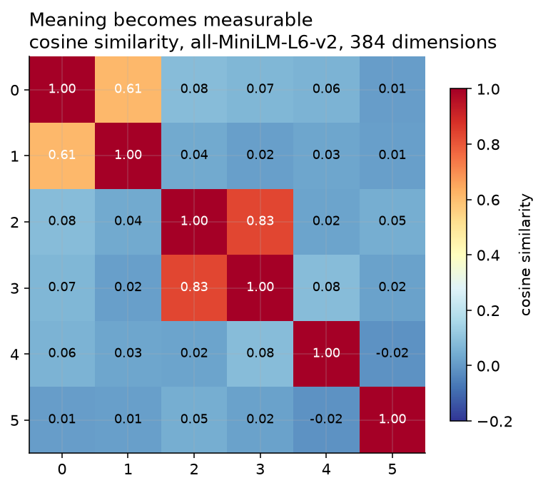
Figure 1:Cosine similarity between six sentences, measured with all-MiniLM-L6-v2 in 384 dimensions.
Row and column 0 is “The cat sat on the mat.”, 1 is “A kitten rested on the rug.”, 2 is
“Bakersfield is in Kern County, California.”, 3 is “Kern County’s largest city is
Bakersfield.”, 4 is “The stock market fell sharply on Tuesday.”, and 5 is “Photosynthesis
converts light into chemical energy.” The diagonal is 1.00 because every sentence is identical
to itself. The two bright off-diagonal cells are the two pairs that mean nearly the same thing.
The figure prints two decimal places and the code output above prints three, so the same cell
reads 0.61 here and 0.612 there. Neither is more accurate; they are the same measured number
shown to different precision. Produced by lab/make_figures.py from
lab/out/we5_embeddings.json.
Four facts are visible in that table, and each one is worth stating out loud.
The diagonal is all 1.000. Row 0 against column 0, row 1 against column 1, and so on. Every sentence is perfectly similar to itself, because comparing a vector with itself gives a cosine of 1 by Formula 9.4 with . This is the first thing to check on any similarity matrix you are handed. A diagonal that is not 1 means the vectors were not normalised, or something worse.
The matrix is symmetric. The value at row 2, column 3 is 0.833, and so is the value at row 3, column 2. That has to be true, because Formula 9.3 gives the same answer whichever vector you call . Half the table is therefore a mirror of the other half, and only 15 of the 36 numbers carry new information. Here is that count. The table has 6 rows and 6 columns, so it holds numbers. Six of them are on the diagonal and are all 1.000, which tells you nothing you did not already know, leaving . Those 30 come in mirrored pairs, one above the diagonal and its twin below, so the number of different values among them is .
Rows 2 and 3 score 0.833, the highest pair. Those are the two Bakersfield sentences. They share three important words, “Bakersfield”, “Kern” and “County”, and they arrange them into two different claims. The model scored them as the closest pair in the set, which matches what a person would say.
Rows 0 and 1 score 0.612 while sharing no content words at all. This is the number that argues for the whole approach. “The cat sat on the mat.” and “A kitten rested on the rug.” have “the”, “on” and “a” in common and nothing else. Cat is not kitten. Sat is not rested. Mat is not rug. A method that counts shared words scores that pair near zero. The embedding scores it 0.612, because the model is comparing meaning rather than spelling.
Rows 4 and 5 score -0.017, which is below zero. “The stock market fell sharply on Tuesday.” against “Photosynthesis converts light into chemical energy.” The cosine went negative. Section 9.4 already put that in proportion: -0.0166 is an angle of 90.95 degrees, which is under one degree past a square corner. It means “nothing to do with each other”, not “these two contradict”.
9.6 Changing one thing at a time
This section carries the course’s Upper Division Area 5 element 6, “experimental controls and data interpretation”. It also sets up Chapter 11.
Intuition
Suppose you bake two loaves of bread. For the second one you use a different flour, and you also leave it in the oven ten minutes longer. The second loaf comes out better. Which change made it better?
You cannot say. Not “you are not sure”. You genuinely cannot say, and no amount of staring at the second loaf will tell you, because two things changed at the same time and the loaf only has one outcome. The experiment was spoiled before the oven was switched on. The only repair is to bake again, changing one thing.
That is the whole idea, and it has a name.
Here is why this section sits in a chapter about cosine similarity rather than somewhere in Module E. The three pairs of arrows you have been computing with all chapter are not three unrelated examples. They are a controlled experiment, already run, with the results already in front of you. Nobody pointed that out while you were doing the arithmetic. It is worth seeing now, because this is a small enough experiment to hold in your head, and every later experiment in the course has the same shape and more moving parts.
The mathematics
Lay the four vectors out with their lengths next to them. Every number here has already appeared on this page.
| Vector | Coordinates | Length | Direction compared with | Raw dot product with | Cosine with |
|---|---|---|---|---|---|
| 5 | the same, it is | 25 | 1.0000 | ||
| 10 | the same | 50 | 1.0000 | ||
| 5 | different | 24 | 0.9600 | ||
| 5 | different, a right angle | 0 | 0.0000 |
Read it as two experiments, not one table.
Experiment 1, rows 1 and 2. The direction is held fixed, because lies along the same line as . The length is the one variable that moves, from 5 to 10. Result: the cosine did not move. It is 1.0000 in both rows.
Experiment 2, rows 1, 3 and 4. The length is held fixed, at 5 in all three rows. The direction is the one variable that moves. Result: the cosine moved a great deal, from 1.0000 to 0.9600 to 0.0000.
Those two experiments together are what lets you make a claim that is stronger than “the cosine seems to be about direction”. They let you say: length does not affect the cosine, and direction does. One experiment on its own could not establish that. You need the one where the thing you suspect does not matter is changed and nothing happens, and the one where the thing you suspect does matter is changed and something happens.
Now look at the fifth column, the raw dot product, and read it as a fourth result. In Experiment 1 the dot product moved from 25 to 50. In Experiment 2 it moved from 25 to 24 to 0. The raw dot product responds to both variables. That is the definition of confounded: a dot product of 50 could have come from a longer arrow or a better-aligned arrow, and the number itself cannot tell you which. Cosine similarity is the version of the measurement with the nuisance variable removed.
Formula 9.7: the manipulation ratio
Before you trust the result of an experiment, check that you changed what you meant to change. For a length, that check is one division.
1. In words. Divide the length of the new vector by the length of the original vector. The answer tells you how many times longer the new one is. A value of 1 means the length did not change at all.
2. The formula.
3. The symbols.
| Symbol | How to say it out loud | What it means |
|---|---|---|
| “ar” | the answer: how many times longer is than . It has no units, because a length divided by a length cancels the units. | |
| “equals” | the two sides are the same number. | |
| “the length of b” | the length of the new vector, from Formula 9.2. | |
| “the length of a” | the length of the original vector. | |
| the fraction bar | “divided by” | divide the top by the bottom. |
4. Out loud. “r is the length of b divided by the length of a.”
5. Worked, with every step.
For against :
The length doubled, which is what Experiment 1 intended.
For against :
The length did not change, which is what Experiment 2 needed to be true.
For against :
Also unchanged.
6. Check it. A manipulation ratio is never negative, because both lengths are positive. A ratio of exactly 1 means the variable was successfully held fixed. If you meant to hold length fixed and got a ratio of 1.3, your experiment is confounded and the result cannot be trusted, no matter how clean the rest of the arithmetic looks. The simulation earlier in this chapter shows this ratio in a box of its own for exactly this reason.
Python
This cell computes the whole design table in one pass, including the manipulation ratio, so you can read the experiment as data rather than as prose.
# Cell 9. The controlled comparison, printed as a table: what was held fixed, what moved, what happened.

experiment_vectors = [[3, 4], [6, 8], [4, 3], [-4, 3]]                  # a, then d, then b, then c
experiment_labels = ["a  = (3, 4)", "d  = (6, 8)", "b  = (4, 3)", "c  = (-4, 3)"]

for vector_position in range(4):                          # one row of the table per pass
    one_vector = experiment_vectors[vector_position]
    running_dot = 0                                       # reset all three totals for this row
    squares_of_a = 0
    squares_of_one = 0
    for coordinate_position in range(2):
        running_dot = running_dot + vector_a[coordinate_position] * one_vector[coordinate_position]
        squares_of_a = squares_of_a + vector_a[coordinate_position] ** 2
        squares_of_one = squares_of_one + one_vector[coordinate_position] ** 2
    length_of_a = math.sqrt(squares_of_a)
    length_of_one = math.sqrt(squares_of_one)
    length_ratio = length_of_one / length_of_a            # Formula 9.7, the manipulation check
    cosine_value = running_dot / (length_of_a * length_of_one)        # Formula 9.3
    print(experiment_labels[vector_position],
          " length =", round(length_of_one, 4),
          " length ratio =", round(length_ratio, 2),
          " raw dot =", running_dot,
          " cosine =", round(cosine_value, 4))
Output:
a  = (3, 4)  length = 5.0  length ratio = 1.0  raw dot = 25  cosine = 1.0
d  = (6, 8)  length = 10.0  length ratio = 2.0  raw dot = 50  cosine = 1.0
b  = (4, 3)  length = 5.0  length ratio = 1.0  raw dot = 24  cosine = 0.96
c  = (-4, 3)  length = 5.0  length ratio = 1.0  raw dot = 0  cosine = 0.0
Four columns, and each one answers a different question. Take them one at a time.
The length ratio column is the manipulation check, Formula 9.7. It reads 1.0, 2.0, 1.0, 1.0.
Only row d has a ratio other than 1, so only row d changed the length. Rows b and c held
length fixed at exactly the value row a had. That is the experiment confirming, in data, that
it was set up the way the prose claimed.
The raw dot column reads 25, 50, 24, 0. It moves in every row. It moved when only the length changed, going from 25 to 50, and it moved when only the direction changed, going from 25 to 24 to 0. A single number from this column cannot tell you which variable produced it. That is confounding, printed.
The cosine column reads 1.0, 1.0, 0.96, 0.0. It did not move for row d, where only length
changed. It moved for rows b and c, where only direction changed. One column responds to both
variables and the other responds to one. That contrast is the whole result.
Check the two columns against each other for row d. The raw dot product doubled, from 25 to 50,
and the length ratio says why: the arrow doubled. The cosine did not move at all. Nothing was
hidden and nothing was smoothed over; the doubling is visible in two columns and absent from the
third, which is what “we removed that variable” looks like when you print it.
Where this goes next
Two later results in this course are controlled experiments in exactly the sense defined above, and both are worth seeing now so you can recognise the shape when it arrives.
The size ladder, in Chapter 11. Three models are compared: Qwen2.5-0.5B, Qwen2.5-1.5B and
Qwen2.5-3B. One model family, so the training recipe is held fixed. One question bank of twenty
questions, so the test is held fixed. One scoring procedure, applied identically, so the marking
is held fixed. The only variable that moves is the parameter count: 494,032,768, then
1,543,714,304, then 3,085,938,688. Their scores under the rotation-debiased procedure were
15.0 per cent, 70.0 per cent and 95.0 per cent, with standard errors of 0.0798, 0.1025 and
0.0487 (real, from lab/out/lab4_size_ladder.json, which stores the three scores as the
decimals 0.15, 0.7 and 0.95; multiplying each by 100 is what turns them into the percentages
printed here). A standard error is the measure of how far a score like this would be expected to
wander if you asked a different twenty questions; Chapter 12 builds it from zero and turns it
into an interval.
Now say carefully what the design does and does not buy you. Because everything else was held
fixed, size is the only variable left that could have produced the rise, so if the rise is
real then size is what caused it. That is what a controlled design gives you and it is worth a
great deal. What it does not give you is the “if”. Twenty questions is a small test, and the
course’s own paired analysis of the top two rungs finds that a gap of 95.0 against 70.0 does
not reach the usual bar for calling a difference settled: the exact test built for this
design returns , which is above 0.05 (real, from
lab/out/appendix_formulas_checks.json, paired_vs_unpaired.mcnemar_exact_p). The letter
there is a number between 0 and 1, and the rough reading is “how easily luck alone could have
produced a gap this big”. The convention people use is that below 0.05 counts as settled,
and 0.0625 is above it, so this one does not count. That convention is a habit rather than a law
of nature, and Chapter 12 works through both the number and the habit. Hold both halves at once: the design is clean, and the test is still too
small to settle the question. Had the three models come from three different families, even a
clean result would have told you nothing about size.
The retrieval arc, in Chapter 10. Three passes over the same corpus of CSUB documents. The
first used fixed-width text windows and essentially never found the right section. The second
changed one thing, the way the text was cut into chunks, and got 3 of 6 questions right. The
third changed one more thing, the embedding model, and got 6 of 6 (real, from
_research/00-lab-verified-findings.md, section 11, produced by lab/lab2_rag_v2.py and
lab/lab2_rag_v3.py). Because each pass changed one thing, each improvement can be attributed
to the thing it changed.
“3 of 6” is a proportion: a count of successes written next to the count of attempts. Turned into a single number it is , and as a percentage that is per cent. This course writes the two counts rather than the percentage, because “50 per cent” hides how few attempts there were and “3 of 6” does not. See Math Toolkit section 12. Six questions is an even smaller test than twenty, so read 3 of 6 and 6 of 6 as the direction of a result and not as its size. The design is what is being taught here; Chapter 12 is where the size of a result gets its interval.
And Chapter 10 carries a sting that belongs to this section. The better system, the one that got 6 of 6, had a smaller average gap between its first and second results, 0.055 against 0.058, than the worse system that got 3 of 6 (real, same source). A gap is a useful confidence signal within one system and it does not transfer across systems. Holding one variable fixed lets you compare. Changing the system underneath a diagnostic and then comparing the diagnostic does not.
Common mistakes
These are the eight things that go wrong most often. Each one comes with a way to spot it.
1. Forgetting a square root when computing a length. You add the squares and use that total as the length, skipping . How to spot it: the cosine comes out far too small. For and the bottom of the fraction should be , and without the roots it becomes , so the answer is instead of . The check: the length of a vector must be at least as big as its largest coordinate ignoring sign. For a length of 25 is impossible; it has to be 5.
2. Dividing by one length instead of both. How to spot it: the answer lands outside -1 to 1. For and , dividing 50 by only 5 gives 10, which is not a cosine of anything. The check: every cosine similarity is between -1 and 1, with no exceptions ever.
3. Reading cosine similarity as a distance. A distance is small when two things are alike. Cosine is large when two things are alike. How to spot it: you find yourself saying “the cosine distance is 0.833” or ranking results smallest-first. The check: a sentence compared with itself gives 1, the top of the scale. If your measure gives 0 for a sentence against itself, it is a distance and not a cosine.
4. Treating a negative cosine as a contradiction. A cosine of -0.017 is an angle of 90.95 degrees, which is under one degree past a square corner. It means unrelated, not opposite. How to spot it: you write a sentence claiming a model detected that two texts disagree. The check: convert the cosine to an angle with Formula 9.5. A genuine opposite would be near -1 and near 180 degrees.
5. Resetting the running totals in the wrong place. In a loop inside a loop, the totals must be set back to 0 at the top of every pass of the outer loop. How to spot it: the first answer is right and every answer after it is too big. The check: compute the first two rows by hand and compare.
6. Comparing vectors of different dimensions. Every position in one vector needs a partner in
the other. A 384-number vector cannot be dotted with a 768-number vector. How to spot it:
Python raises an error mentioning shapes. The check: print .shape on both before you compare
them.
7. Rounding before computing rather than after. Rounding a cosine to two decimal places and then taking the arccos gives a different angle from rounding at the end. How to spot it: your angle disagrees with a printed one in the first decimal place. The check: carry full precision through every step and round only the thing you print. See Math Toolkit section 16.
8. Drawing a conclusion from a comparison in which two things changed. The commonest mistake in this whole course, and the only one on this list that no arithmetic will catch. How to spot it: write down every variable that differed between your two conditions. If the list has more than one entry, stop. The check: Formula 9.7 and its relatives. Confirm that the variables you meant to hold fixed really did stay fixed, and say so in writing.
What to remember
Cosine similarity is the dot product of two vectors divided by both of their lengths, and it always lands between -1 and 1. Dividing by the lengths removes length from the answer and leaves direction, which is the part that carries meaning, and the proof is that and score exactly 1.0000 because the second is the first doubled. The same arithmetic runs unchanged in 384 dimensions, where two sentences about Bakersfield and Kern County score 0.8333, a cat and a kitten score 0.6124 while sharing no content words, and two unrelated sentences go slightly below zero at -0.0166. Normalising both vectors to length 1 first makes the cosine identical to a plain dot product, which is why the code is one line. And no comparison in this course is worth reporting unless exactly one variable moved and every other variable was held fixed on purpose.
Practice problems
Twenty-eight problems in three tiers. Warm-up asks whether you can do the arithmetic. Practice asks whether you can apply it. Stretch asks whether you can reason with it. Answers to the odd-numbered problems are in the answers appendix.
Every vector in these problems is made up for practice unless the problem says it comes from the lab. Show every step, the way the worked examples do.
Warm-up
1. Work out the dot product of and .
2. Work out the dot product of and . What does your answer say about the angle between them?
3. Work out the length of .
4. Work out the length of , to six decimal places.
5. Work out the length of .
6. Work out the length of . This one comes out whole.
7. Work out the cosine similarity of and .
8. Work out the cosine similarity of and . Predict the answer before you compute it.
9. Work out the cosine similarity of and .
10. Which of these four numbers could be a cosine similarity, and which could not: 1.4, -0.017, 0.833, -2? Give the reason in each case.
Practice
11. Work out the cosine similarity of and , showing all five steps.
12. Work out the cosine similarity of and , to four decimal places.
13. Take the vector and scale it by . Write down the new vector, its length, and its cosine similarity with the original. Predict all three before computing any of them.
14. Take the vector and scale it by . Work out the cosine similarity with the original. Explain the sign of your answer in one sentence.
15. The two Bakersfield sentences in this chapter have a measured cosine similarity of 0.8333. Convert it to an angle in degrees.
16. The cat sentence and the kitten sentence have a measured cosine similarity of 0.6124. Convert it to an angle in degrees. Then state, in one sentence, whether the angle or the cosine makes the two sentences look more different, and why that is a fact about units rather than about the sentences.
17. Normalise the vector by hand. Give both coordinates to four decimal places, then check that the length of your answer is 1.
18. A classmate computes the cosine similarity of and and gets 10. Find their mistake without redoing the whole calculation, using only the sanity checks in this chapter.
19. Using the similarity matrix printed in Section 9.5, list the three lowest off-diagonal values in the table and say which sentence pairs they belong to.
20. Two vectors have already been normalised to length 1. Their dot product is 0.7. What is their cosine similarity, and how do you know without dividing by anything?
21. A student wants to compare two embedding models on the same six sentences. Write down three variables they must hold fixed and one variable they should change.
Stretch
22. Show, using Formula 9.3 and nothing else, that the cosine similarity of any non-zero vector with itself is exactly 1. Do it with letters, not with particular numbers.
23. Show that the cosine similarity of with is exactly -1, for any non-zero . Use the general argument in Section 9.3 as your model.
24. Explain in your own words why the similarity matrix in Section 9.5 must be symmetric. Your explanation should refer to a specific feature of Formula 9.3.
25. A search system ranks passages by raw dot product with the question, using un-normalised embeddings. Describe the systematic bias this creates, name which kind of passage benefits, and say what single change fixes it.
26. The chapter says that a cosine of -0.0166 and a cosine of +0.0166 are both best read as “unrelated”. Support that claim with two arccos computations, and then say what would have to be true of a cosine before you would be willing to call two texts genuinely opposite.
27. Cosine similarity cannot tell apart from , or from . Describe one situation in which throwing away the length is exactly right, and one situation in which it would lose information you needed. Be specific about what the length would have meant in your second situation.
28. Chapter 10 reports that the better retrieval system had a smaller average gap between its first and second result, 0.055 against 0.058, than the worse system. Using the vocabulary of Section 9.6, explain why this does not mean the gap is a useless diagnostic, and state the exact condition under which comparing two gaps is legitimate.
Where to go next
Chapter 10, Retrieval: the open-book exam takes the measure you built here and sorts with it. Give a model a question, score the question against every passage in a corpus of real CSUB and Kern County documents, and hand the model the passage that scored highest. That is the whole architecture, and it works exactly as well as the cosine similarities underneath it.
If any formula on this page is still not settled, the Formula Sheet sets out four of the seven again in the same six parts, as entries 5.1 to 5.4: the dot product, the length of a vector, cosine similarity, and the angle from a cosine. Its entry 5.5 is the retrieval rule Chapter 10 needs. The Math Toolkit has every symbol on this page from zero, and its Formulas 15 and 17 are this chapter’s Formulas 9.1 and 9.2 written a second way.