1Objectives
By the end of this lesson you will be able to:
Run and interpret a Welch two-sample t-test with
t.test(y ~ g, data=).Run and interpret a paired t-test with
t.test(~diff, data=).Run and interpret a two-proportion test with
prop.test(c(x1,x2), c(n1,n2)).Run and interpret a chi-square test of independence with
xchisq.test(tally(y ~ x, data=)), including its observed/expected/residual display.Read back every test’s decision in one plain-language sentence.
2From one group to two (or more)
L10 built the logic of a hypothesis test — state and
, check conditions, compute a test statistic and a p-value, decide —
and already put two comparisons to work: a Welch two-sample t.test(y ~ g, data=) (cat people vs. dog people’s sleep) and a two-proportion
prop.test(c(x1,x2), c(n1,n2)) (cat-person rate, Freshmen vs. Sophomores).
This lesson keeps that exact logic, gives you one more worked example of
each so the pattern sticks, and adds the two shapes of comparison L10 didn’t
reach yet — paired measurements and categorical association:
| Comparison | R function | New here, or practice from L10? |
|---|---|---|
| Two independent group means | t.test(y ~ g, data=) (Welch two-sample) | Practice — new example |
| Two paired measurements on the same subjects | t.test(~diff, data=) | New |
| Two group proportions | prop.test(c(x1,x2), c(n1,n2)) | Practice — new example |
| Association between two categorical variables | xchisq.test(tally(y ~ x, data=)) | New |
Reload the running dataset if you’re starting fresh:
suppressMessages({library(mosaic); library(BSDA)})
set.seed(2200)
survey <- read.csv("data/survey_sim.csv")
survey$class_year <- factor(survey$class_year,
                             levels = c("Freshman", "Sophomore", "Junior", "Senior"))
survey$pet <- factor(survey$pet, levels = c("Cat person", "Dog person", "Neither"))
survey$major_area <- factor(survey$major_area)
read.csv() reads class_year, pet, and major_area in as plain text
(L06); wrapping each in factor() (with levels = spelling out
Freshman-before-Sophomore-before-Junior-before-Senior order for class_year)
is what lets L07’s tables print in that logical order instead of
alphabetical, and is what makes Section 1’s droplevels() meaningful below.
31. Welch two-sample t-test: comparing two independent means
Independent samples means the two groups are made of different
students — no student appears in both. Are Exam 1 scores different for STEM
majors versus Business majors? Start with EDA, restricting survey to just
those two majors:
sub2 <- subset(survey, major_area %in% c("STEM", "Business"))
sub2$major_area <- droplevels(sub2$major_area)   # drop the unused major levels
favstats(exam_score ~ major_area, data = sub2)
major_area min Q1 median Q3 max mean sd n missing
1 Business 42.2 56.150 60.3 66.40 76.7 60.88065 8.811145 31 0
2 STEM 39.7 54.375 58.0 67.85 80.7 60.57917 10.646819 24 0droplevels() matters here: major_area still remembers its other three
levels (Nursing, Kinesiology, Other) even after subset() removes every row
that had them. Without droplevels(), favstats(exam_score ~ major_area, data = sub2) would print all five majors — three of them with n = 0 and
NaN for every statistic — because it still believes those empty levels
exist. Dropping the unused levels first keeps the output to the two majors
that actually have data.
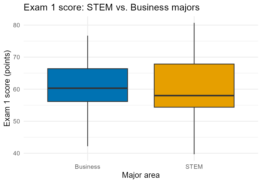
Figure 1:Exam 1 score, STEM vs. Business majors — a quick EDA look before testing.
The two groups’ means (60.9 vs. 60.6) are close, and the boxes overlap
almost completely — EDA already hints this comparison won’t turn up much.
Test it the same way L10 tested sleep_hours ~ pet:
t.test(exam_score ~ major_area, data = sub2)
	Welch Two Sample t-test

data:  exam_score by major_area
t = 0.11214, df = 44.307, p-value = 0.9112
alternative hypothesis: true difference in means between group Business and group STEM is not equal to 0
95 percent confidence interval:
 -5.115581  5.718538
sample estimates:
mean in group Business     mean in group STEM
              60.88065               60.57917
: vs. : . With and — nowhere near a typical — fail to reject . The 95% CI for the difference in means, , contains 0, telling the same story: this sample gives no evidence that STEM and Business majors score differently on Exam
Same title, same “Welch” default, same reasoning as L10’s example — different pair of groups.
42. Paired t-test: comparing two measurements on the same subjects
Paired data means each subject is measured twice, and you care about
the within-subject change — the opposite setup from Section 1’s two
separate groups. R ships a classic paired-data example built in, no import
needed (same idea as faithful in L06): sleep, ten patients
each given two drugs, with extra recording each patient’s extra hours of
sleep on that drug.
data(sleep)
str(sleep)
'data.frame': 20 obs. of 3 variables:
$ extra: num 0.7 -1.6 -0.2 -1.2 -0.1 3.4 3.7 0.8 0 2 ...
$ group: Factor w/ 2 levels "1","2": 1 1 1 1 1 1 1 1 1 1 ...
$ ID : Factor w/ 10 levels "1","2","3","4",..: 1 2 3 4 5 6 7 8 9 10 ...Twenty rows, but only ten patients (ID 1–10) — group 1 is Drug 1’s
measurement and group 2 is Drug 2’s, per patient. That’s the giveaway for
paired data: the same ID shows up twice. t.test(~diff, data=) needs the
difference already computed as one column, so reshape to one row per
patient first:
sleep_wide <- reshape(sleep, timevar = "group", idvar = "ID", direction = "wide")
sleep_wide$diff <- sleep_wide$extra.2 - sleep_wide$extra.1
sleep_wide
ID extra.1 extra.2 diff
1 1 0.7 1.9 1.2
2 2 -1.6 0.8 2.4
3 3 -0.2 1.1 1.3
4 4 -1.2 0.1 1.3
5 5 -0.1 -0.1 0.0
6 6 3.4 4.4 1.0
7 7 3.7 5.5 1.8
8 8 0.8 1.6 0.8
9 9 0.0 4.6 4.6
10 10 2.0 3.4 1.4extra.1 and extra.2 are Drug 1’s and Drug 2’s readings for that same
patient, side by side; diff is Drug 2 minus Drug 1. Look at diff the way
L07 taught — favstats() on it first:
favstats(~diff, data = sleep_wide) min Q1 median Q3 max mean sd n missing
0 1.05 1.3 1.7 4.6 1.58 1.229995 10 0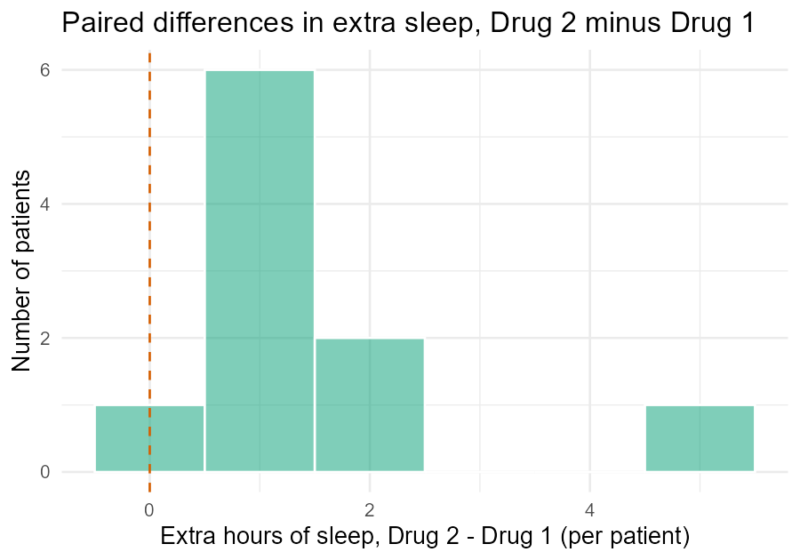
Figure 2:Paired differences (Drug 2 - Drug 1), the built-in sleep dataset.
Every one of the ten differences is at or above zero — a strong visual hint before any test that Drug 2 tends to add more sleep. A paired t-test is just a one-sample t-test on the differences, testing :
t.test(~diff, data = sleep_wide)
	One Sample t-test

data:  diff
t = 4.0621, df = 9, p-value = 0.002833
alternative hypothesis: true mean is not equal to 0
95 percent confidence interval:
 0.7001142 2.4598858
sample estimates:
mean of x
     1.58
, well under : reject . The 95% CI for
the mean difference, hours, does not contain 0 — consistent
evidence that Drug 2 is associated with more extra sleep than Drug 1 in this
sample, averaging about 1.58 extra hours. Notice ~diff is a
one-sided formula (nothing on the left of ~) — the same “just one
variable” shape L06 and L07 used for favstats(~x, data=), because after reshaping there is only one variable (the
difference) left to test.
53. Two-proportion test: comparing two group proportions
L10 already ran prop.test(c(x1,x2), c(n1,n2)) once, comparing
the cat-person rate between Freshmen and Sophomores. Here’s a second
question, same tool: L07 found that more study time went with
higher exam scores. Turn that into a yes/no question — are students who
study at or above the class median more likely to pass Exam 1 (score
) than students who study below it?
med <- median(~study_min, data = survey)
survey$pass <- ifelse(survey$exam_score >= 60, "Pass", "Not yet")
survey$study_grp <- factor(ifelse(survey$study_min >= med,
                                   "High study time", "Low study time"),
                            levels = c("Low study time", "High study time"))
tally(pass ~ study_grp, data = survey)
study_grp
pass Low study time High study time
Not yet 35 18
Pass 25 42prop.test() wants raw counts, not a table — pull the “successes” (, the
Pass count) and totals () for each group:
hi <- subset(survey, study_grp == "High study time")
lo <- subset(survey, study_grp == "Low study time")
x1 <- sum(hi$pass == "Pass");  n1 <- nrow(hi)    # 42 of 60
x2 <- sum(lo$pass == "Pass");  n2 <- nrow(lo)    # 25 of 60
prop.test(c(x1, x2), c(n1, n2))
	2-sample test for equality of proportions with continuity correction

data:  c out of cx1 out of n1x2 out of n2
X-squared = 8.6511, df = 1, p-value = 0.003269
alternative hypothesis: two.sided
95 percent confidence interval:
 0.09635351 0.47031316
sample estimates:
    prop 1     prop 2
0.7000000 0.4166667
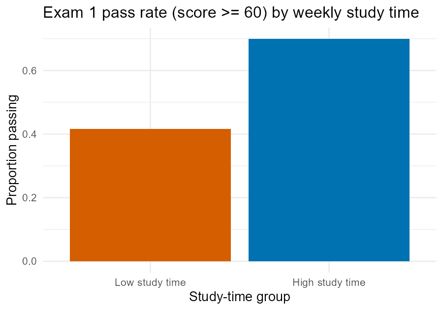
Figure 3:Exam 1 pass rate by weekly study-time group.
: the two groups’ true pass rates are equal; : they differ.
X-squared = 8.65, p = 0.0033 — reject . prop 1 (0.70, the
high-study-time group, since c(x1, x2) listed it first) and prop 2
(0.417, low-study-time) are the two sample proportions being compared; the
95% CI for their difference, , does not include 0. In this
sample, studying at or above the class median goes with a meaningfully
higher Exam 1 pass rate.
64. Chi-square test of independence: two categorical variables
L07 built a two-way tally() of pet preference by class year and
eyeballed that the proportions looked “fairly stable across years.” A
chi-square test of independence turns that eyeball check into a formal
decision: : pet preference and class year are independent (unrelated);
: they’re associated. Start from the exact same table:
tab <- tally(pet ~ class_year, data = survey)
tab
class_year
pet Freshman Sophomore Junior Senior
Cat person 9 14 11 6
Dog person 16 11 16 12
Neither 5 11 6 3mosaic’s xchisq.test() runs the same test as base R’s chisq.test() but
also prints every cell’s expected count and residual — exactly the
diagnostic detail you need to say why a result came out the way it did:
xchisq.test(tab)
	Pearson's Chi-squared test

data:  x
X-squared = 5.8412, df = 6, p-value = 0.4412

    9       14       11        6
(10.00)  (12.00)  (11.00)  ( 7.00)
[0.100]  [0.333]  [0.000]  [0.143]
<-0.32>  < 0.58>  < 0.00>  <-0.38>

   16       11       16       12
(13.75)  (16.50)  (15.12)  ( 9.62)
[0.368]  [1.833]  [0.051]  [0.586]
< 0.61>  <-1.35>  < 0.22>  < 0.77>

    5       11        6        3
( 6.25)  ( 7.50)  ( 6.88)  ( 4.38)
[0.250]  [1.633]  [0.111]  [0.432]
<-0.50>  < 1.28>  <-0.33>  <-0.66>

key:
	observed
	(expected)
	[contribution to X-squared]
	<Pearson residual>
Read the grid one cell at a time using the key: at the bottom — for
Freshman/Cat person: 9 students observed, (10.00) expected if pet
preference and class year were truly unrelated, a [0.100] share of the
total chi-square statistic coming from that one cell, and a Pearson
residual of -0.32 (observed a bit below expected; residuals beyond about
are the ones worth a second look — none here come close).
X-squared = 5.84, df = 6, p = 0.4412: fail to reject . No
cell’s residual stands out, and the p-value confirms it — this sample gives
no evidence that pet preference and class year are related, matching
L07’s informal read exactly.
7Summary
t.test(y ~ g, data=)runs a Welch two-sample t-test on independent groups;droplevels()a grouping factor first if it has unused levels left over from asubset().t.test(~diff, data=)runs a paired t-test — a one-sample test on a difference column you compute first (e.g., viareshape()on wide/long data with a shared ID, as with the built-insleepdataset).prop.test(c(x1,x2), c(n1,n2))compares two group proportions; pull the successes (x1,x2) and totals (n1,n2) from atally()first.xchisq.test(tally(y ~ x, data=))tests whether two categorical variables are associated, and prints observed counts, expected counts, each cell’s contribution to X-squared, and Pearson residuals — read them with thekey:at the bottom of the output.Every test here follows the same decision logic as L10: state /, check the test’s conditions, read the p-value against , decide, and say what that decision means in one plain sentence.
The full script that generated every figure and every number in this lesson is committed at
data/make_L11_figures.R— run it yourself to reproduce all of it exactly.