Last week you built your first probability distribution table and used it to find a game’s expected winnings — the long-run average payout if you played over and over. That average is only half the story. Two games can share the exact same average payout and still feel completely different to play: one might pay out close to that average almost every time, while the other swings wildly between a big loss and a rare big win. This week you’ll learn to measure that swing with the standard deviation of a random variable. Then you’ll take the first step past distributions built from a short list of outcomes — discrete random variables — into the kind where the outcome could be any number in a range at all, like a person’s height or how long a coffee order takes. That’s a continuous random variable, and it’s the introduction to the bell-shaped Normal curve you’ll spend the next several weeks with.
1The mean of a random variable, one more time
A random variable assigns a number to every outcome of a random process. Its probability distribution lists each possible value next to , the chance that value occurs — every is between 0 and 1, and they all add up to 1. You already met the mean, or expected value, of :
Read this as a weighted average: instead of averaging every value equally, multiply each value by how likely it is, then add the products. isn’t necessarily a value can even take on — it’s the distribution’s balancing point, and its most useful meaning is a long-run average: if the random process repeated itself thousands of times, the average of all those outcomes would settle in near .
2How far from the mean? The standard deviation of a random variable
The standard deviation of a random variable, written or , measures the typical distance an outcome lands from :
Read it left to right: find each outcome’s deviation from the mean, (this can be negative); square every deviation so negatives don’t cancel positives; weight each squared deviation by its probability and add them up (this sum is the variance, ); then undo the squaring with a square root so comes back in the same units as .
Worked Example 1 — a warm-up with round numbers. Before the richer example below, try the formula on the simplest possible game: flip one fair coin. Heads (probability 0.5) pays $4; tails (probability 0.5) pays $0. Let be the payout.
| Outcome | ||||||
|---|---|---|---|---|---|---|
| Heads | $4 | 0.5 | 2 | 2 | 4 | 2 |
| Tails | $0 | 0.5 | 0 | −2 | 4 | 2 |
| Total | 1.0 | 2 | 4 |
: the long-run average payout is $2. Summing the last column gives the variance, , so . Every step is a round number here on purpose, so you can check each one in your head before the next example makes the numbers messier.
Worked Example 2 — expected winnings on a raffle ticket. A campus club sells 200 tickets at $5 each for a fundraiser. One ticket wins a $300 grand prize, four tickets win a $25 gift card, and the remaining 195 tickets win nothing. Let be a ticket buyer’s net winnings — the prize won minus the $5 cost — for a single ticket.
| Outcome | ||||||
|---|---|---|---|---|---|---|
| Grand prize | $295 | 0.005 | 1.475 | 298 | 88,804 | 444.02 |
| Gift card | $20 | 0.020 | 0.400 | 23 | 529 | 10.58 |
| No prize | −$5 | 0.975 | −4.875 | −2 | 4 | 3.90 |
| Total | 1.000 | −3.00 | 458.50 |
Summing the column gives . On average, a ticket buyer loses $3 per ticket in the long run. That is exactly why the fundraiser works: multiply that average loss by all 200 tickets sold, and for players collectively — which means $600 raised for the club. You can check that number directly, ticket by ticket, instead of through the probability table:
| Amount | |
|---|---|
| Ticket sales (200 tickets × $5) | $1,000 |
| Prizes paid out ($300 + 4 × $25) | $400 |
| Net raised for the club | $600 |
Both routes agree: $600. Summing the last column of the first table and taking the square root gives
A single ticket’s outcome typically lands about $21.41 away from that average — a large spread relative to the mean. Almost every ticket loses exactly $5 (close to average), but the rare $295 win sits far out and pulls the typical distance from the mean way up. A hypothetical raffle with the same mean where every ticket simply lost $3 for certain would have — no spread, because there’d be nothing uncertain about the outcome. Here signals real risk: most players lose a little, a few win a lot.
3From discrete to continuous: density curves
Every random variable so far — carnival-game payouts, raffle winnings — has been discrete: a short list of possible values you can put in a table and add up. Many real quantities aren’t like that. A person’s height, an espresso machine’s steaming time, or a commute can fall anywhere along a continuum, with no useful way to list “every possible value” one at a time. These are continuous random variables, and they need a different tool than a probability table: a density curve.
A density curve is a smooth curve where area, not height, equals probability. The probability that falls between two values and is the area under the curve between and — never read a probability directly off the curve’s height. Two properties always hold: the curve never dips below 0, and the total area under the entire curve equals 1 (some outcome always happens). One especially important density-curve shape — the one you’ll use for the rest of the semester — is the Normal curve: bell-shaped, symmetric, single-peaked, centered exactly at the mean , with its spread controlled by . A Normal curve with mean and standard deviation is written .
Worked Example 3 — Reading area under a density curve. Suppose adult female height (inches) is
modeled by a Normal density curve — a common illustrative figure for this bell shape,
not a claim about any specific real survey. What’s the probability a randomly selected woman is
between 63 and 66 inches tall? Because is continuous, this probability is the area under the
curve between 63 and 66, not a height read off the curve. R’s xpnorm() function computes that area
(quietly converting each boundary to a standardized distance from the mean behind the scenes — a
preview of the z-score tool coming in Week 6) and reports:
so the strip between them has area — about 45.1% of adult women, under this model, fall in that six-inch window. Two things this previews: first, already includes everything up through 63, so the middle strip’s area is the difference of two “less-than” areas — the same whole-minus-the-rest logic you’ll use constantly with density curves. Second, because a single exact height is a line with zero width, the area above any one exact value is 0, so even though .
See it in R.
library(mosaic)

# Worked Example 2: raffle net winnings ($5 ticket, 200 sold)
x <- c(295, 20, -5)             # net winnings (prize won - $5 cost)
p <- c(0.005, 0.020, 0.975)     # 1 grand prize, 4 gift cards, 195 no-prize / 200
sum(p)                          # check: probabilities sum to 1

mu <- sum(x * p)                # E(X)
mu

sigma <- sqrt(sum((x - mu)^2 * p))   # SD(X)
sigma

# Worked Example 3 preview: area under a density curve
xpnorm(c(63, 66), mean = 64.5, sd = 2.5, plot = FALSE)
gf_dist("norm", mean = 64.5, sd = 2.5)   # draws the N(64.5, 2.5) density curve
Running this prints mu = -3 and sigma = 21.41261 — matching the by-hand table above — and
xpnorm() prints P(X ≤ 63) = 0.2743 and P(X ≤ 66) = 0.7257, the same two areas used in Worked
Example 2. gf_dist("norm", ...) draws the density curve itself, a visual check that
it’s bell-shaped and centered where you’d expect.
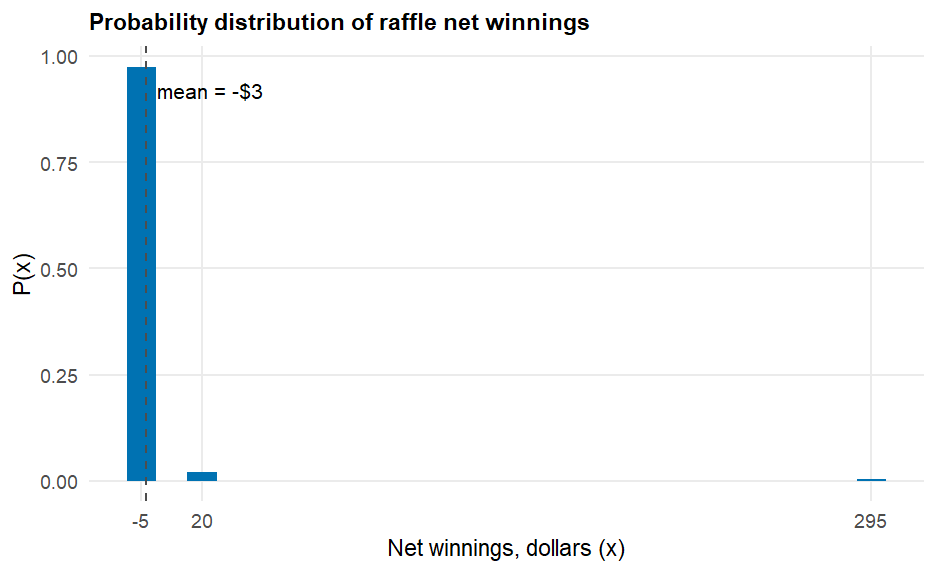
Figure 1. A probability histogram of the raffle’s net winnings has three bars: a very tall bar at reaching a height of 0.975, a short bar at with height 0.02, and a barely visible bar at with height 0.005. A vertical dashed line marks the mean, , sitting just to the right of the tall bar — most tickets lose close to the average, while the rare $295 win sits far out in the right tail and pulls the standard deviation up to $21.41.
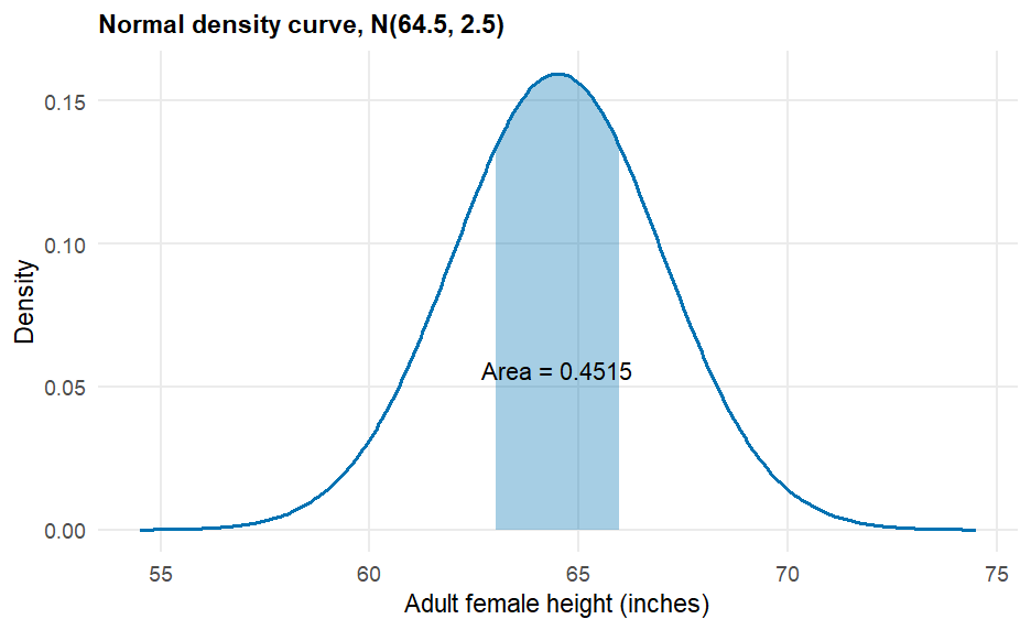
Figure 2. A bell-shaped Normal density curve is shaded between and . The shaded strip’s area, 0.4515, is printed in the middle of the curve; the unshaded area in both tails together equals , and the entire shaded-plus-unshaded region under the curve sums to exactly 1.
4Check your understanding
A carnival ring-toss game costs $3 to play. You win a $10 prize with probability 0.10, a $5 prize with probability 0.20, and nothing the rest of the time. Let be your net winnings. Find .
Using the same ring-toss game, find . (Hint: build the same six-column table as Worked Example 2.)
In Worked Example 2’s raffle, the club sells all 200 tickets. Using , find the players’ total expected net winnings across all 200 tickets, and explain what that number means for the club’s fundraiser.
In Worked Example 3, . Using the fact that the total area under any density curve equals 1, find without computing a new area from scratch.
Explain, in your own words, why height needs a density curve instead of a probability table like the ones you built for discrete random variables in Weeks 4–5.
True or false, with a one-sentence reason: for the continuous in Worked Example 3, .
5Key terms
Random variable () — a variable that assigns a number to every outcome of a random process.
Expected value / mean of a random variable (, ) — the probability-weighted average of a random variable’s possible values, ; best interpreted as a long-run average over many repetitions.
Weighted average — an average in which some values count more than others because they’re multiplied by a weight (here, a probability) before summing.
Deviation — how far a value sits from the mean, ; can be positive or negative.
Variance () — the probability-weighted average of the squared deviations, .
Standard deviation of a random variable (, ) — the square root of the variance; the typical distance an outcome falls from , in the same units as .
Continuous random variable — a random variable that can take any value along a continuum (no gaps), so its possible values can’t be listed in a table.
Density curve — a smooth curve describing a continuous random variable, where area under the curve equals probability; the curve is never negative, and the total area under it always equals 1.
Normal distribution, — a specific bell-shaped, symmetric, single-peaked density curve centered at with spread controlled by .