The student government’s fall fundraiser sets up a table outside the union: a $2 raffle ticket next to it, and the campus coffee cart’s “lucky card” promotion — draw one card from a shuffled deck, win a free drink if it’s a heart. Both games raise the same question a smart customer should ask before playing: what are my actual chances, and what should I expect to walk away with? Last week you learned to read probability as long-run relative frequency and met the complement rule. This week adds two more building-block rules — for combining probabilities with “or” and with “and” — and introduces a new tool, the random variable, that finally lets you answer the second question: not just “will I win?” but “what’s this worth, on average?”
1Combining events with “or”: the addition rule
Every probability lives on the probability scale: a number from 0 (the event never happens) to 1 (it always happens) — you’ll see this written as a decimal or a percent. Recall from last week that the complement of an event , written , is “ does not happen,” and . This week’s first new idea is combining two events with the word “or.” The union of events and — written — is the event that at least one of them happens.
If and can never happen on the same outcome, they’re called disjoint (or mutually exclusive), and . For disjoint events, probabilities simply add:
If and can happen together, adding double-counts the outcomes where both occur, so the general addition rule subtracts that overlap once:
Here is the joint probability that both events happen at once.
Worked Example 1 — the coffee cart’s lucky-card game. The cart uses a standard, well-shuffled 52-card deck; a customer draws one card, and every card is equally likely ( each). Let = “the card is a heart” and = “the card is a face card” (jack, queen, or king, in any suit). There are 13 hearts, so . There are 12 face cards, so .
Complement. The probability of not drawing a heart: (75%).
Disjoint case. “Heart or spade” — a single card can’t be both suits at once, so these events are disjoint, and :
General case. “Heart or face card” is different — the jack, queen, and king of hearts belong to both events, so . Simply adding would count those three cards twice, so the general rule subtracts the overlap:
About 42.3% of draws win at least one prize.
Independence and the multiplication rule. Two events are independent if knowing the outcome of one tells you nothing about the other — like two different customers each drawing from their own separately shuffled deck. For independent events, the probability both happen is the product:
So the probability that two independent customers both draw hearts is (6.25%).
The same rule governs any two independent processes, even something as ordinary as two coin
flips. Simulating 1000 pairs of independent fair-coin flips (set.seed(1209)) landed both
heads 261 times out of 1000 — an empirical probability of — close to the
theoretical the multiplication rule predicts; the small gap is exactly the
random noise you’d expect from only 1000 repetitions.
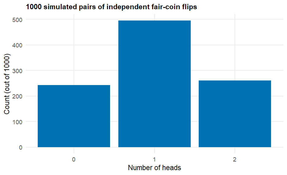
Figure 1. A bar chart of 1000 simulated two-coin-flip repetitions shows three bars — 0 heads, 1 head, 2 heads — at heights 243, 496, and 261 out of 1000. The middle bar (exactly one head) is roughly twice as tall as each outer bar, matching the lopsided-in-the-middle shape the multiplication rule predicts for two independent coins.
2Random variables and probability distributions
A random variable, usually written , assigns a number to the outcome of a random process — dollars won, number of heads, minutes late. A discrete random variable takes on a countable list of specific values (a continuous random variable, coming in two weeks, can take any value in a range). The probability distribution of is a table listing every possible value alongside , the probability equals that value. Because the table lists every possibility and no two rows overlap, a valid distribution always satisfies .
Worked Example 2 — the fundraiser raffle. The raffle sells tickets at $2 each. Prizes: 1 grand prize of $250, 4 prizes of $50, and 20 prizes of $10; the remaining tickets win nothing. Let = the dollar amount a randomly selected ticket wins:
| (dollars won) | |
|---|---|
| 250 | 1/500 = 0.002 |
| 50 | 4/500 = 0.008 |
| 10 | 20/500 = 0.040 |
| 0 | 475/500 = 0.950 |
| Total | 1.000 |
The probabilities sum to exactly 1, confirming this is a valid distribution.
Expected value. The expected value of a discrete random variable is the probability-weighted average of its possible values:
Here means “add up every row,” is each possible value, and is its probability. (also written , “mu”) is the long-run average — not what any single ticket wins, but what the average payout per ticket would settle toward if the same raffle ran over and over. Multiplying and adding row by row:
So . Since a ticket costs $2, the expected net result of playing is per ticket — on average, a player loses about 70 cents per ticket, which is exactly the money that funds the student-government fundraiser. No individual ticket ever actually wins $1.30; the number describes the average over many, many tickets.
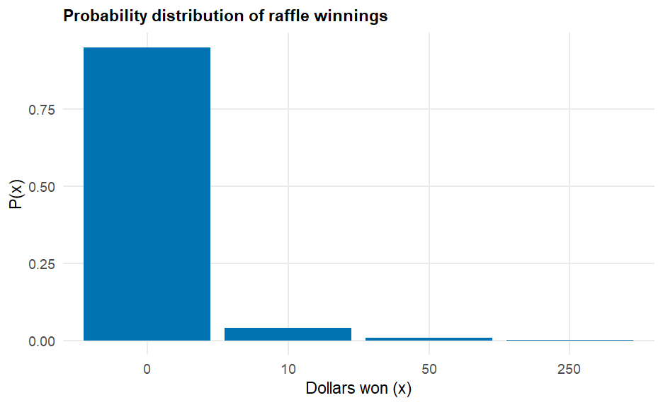
Figure 2. A probability-distribution bar chart for the raffle has four bars at ; the bar at towers to a height of 0.95, while the other three bars are barely visible slivers at 0.04, 0.008, and 0.002 — a strongly lopsided distribution where “win nothing” dominates, even though the rare big prize is what pulls up above zero.
See it in R.
suppressMessages({library(mosaic); library(BSDA)})

# Worked Example 1: probability rules on a standard 52-card deck
p_heart <- 13/52
p_face  <- 12/52
p_heart_and_face <- 3/52                                   # J, Q, K of hearts
p_heart_or_face  <- p_heart + p_face - p_heart_and_face    # general addition rule
p_heart_or_spade <- 13/52 + 13/52                          # disjoint -> simple addition
p_not_heart <- 1 - p_heart                                 # complement rule
p_heart^2                                                   # multiplication rule, independent

# empirical check of the multiplication rule: 1000 pairs of independent fair coins
set.seed(1209)
sim <- do(1000) * rflip(2)
tally(~ heads, data = sim)
mean(~ (heads == 2), data = sim)     # empirical P(both heads)

# Worked Example 2: raffle distribution table and expected value
x <- c(250, 50, 10, 0)
p <- c(1/500, 4/500, 20/500, 475/500)
sum(p)            # check the distribution sums to 1
sum(x * p)         # E(X)
Running tally(~ heads, data = sim) prints exactly the 243 / 496 / 261 counts behind Figure 1, and
sum(x * p) returns 1.3, confirming from Example 2.
3Check your understanding
Using last week’s shelter data, . What is , the probability a randomly chosen intake is not a Large animal? Which rule did you use?
A fair six-sided die is rolled once. Are “rolling a 2” and “rolling a 5” disjoint events? Find .
Using the coffee cart’s deck (Worked Example 1), find . Are these two events disjoint? Show the general addition rule step you used.
Recall from Week 3’s
coffee_simdata that (94 of 300 orders). If two different customers place their orders independently, what is the probability both order a latte?A small carnival ring-toss game charges to play. Let = dollars a player wins, with this distribution:
$5 $1 −$1 0.10 0.30 0.60 (a) Verify this is a valid probability distribution. (b) Find and interpret it in one plain-language sentence.
Worked Example 2 found for the raffle, even though no single ticket can actually win exactly $1.30. Explain what means, using the phrase “long-run average.”
4Key terms
Probability scale — probability is always a number from 0 (never happens) to 1 (always happens).
Complement () — the event “ does not happen”; .
Union (“or”) — the event that at least one of or happens.
Disjoint (mutually exclusive) events — events that cannot both happen on the same outcome, so .
Addition rule (disjoint) — , valid only when and are disjoint.
Addition rule (general) — ; the subtraction removes double-counted outcomes.
Joint probability, — the probability that both and happen.
Independent events — knowing whether one event happened gives no information about the other.
Multiplication rule (independent events) — .
Random variable () — a variable that assigns a number to the outcome of a random process.
Discrete probability distribution — a table of every possible value of a discrete random variable with its probability ; a valid table always has .
Expected value (, or ) — ; the probability-weighted average value of , interpreted as its long-run average over many repetitions.