Week 10 — Confidence Intervals - Statistics in the Modern World (MATH 1209)

This week in one line: you’ll turn a single wobbly point estimate into a confidence interval — a whole range of plausible values, built as point estimate ± margin of error.

Last week you met the point estimate — a single number like $\hat p$ or $\bar x$ , built from one sample, that almost never lands exactly on the true population parameter — and you learned to measure how much that number bounces around from sample to sample with the standard error, $SE$ . A single number with no sense of “how far off could this be” is a weak thing to build a decision on.

This week turns that wobbly point estimate into something far more honest: a confidence interval — a whole range of plausible values for the parameter, built around the point estimate, with a stated confidence level attached to how well the procedure itself performs in the long run.

1Point estimate ± margin of error¶

Every confidence interval has the same skeleton:

\text{point estimate} \ \pm\ \text{margin of error (ME)}

The margin of error is how far, in either direction, the interval reaches from the point estimate. For a large sample, $ME = z^\star \cdot SE$ , where $SE$ is last week’s standard error and $z^\star$ (read “z-star”) is a critical value: a fixed number of standard errors chosen so that the interval-building procedure captures the true parameter a stated percentage of the time. Three critical values come up constantly enough to know by name:

Confidence level	Critical value $z^\star$
90%	1.645
95%	1.960
99%	2.576

A higher confidence level needs a larger $z^\star$ : capturing the truth more often requires casting a wider net.

2A confidence interval for a proportion¶

For a sample proportion $\hat p$ (successes $x$ out of $n$ trials), the large-sample interval is

\hat p \ \pm\ z^\star\sqrt{\dfrac{\hat p(1-\hat p)}{n}}

Worked Example 1 — library hours. CSUB surveys $n=400$ randomly selected students on extending library hours to midnight during finals week; $x=208$ say yes, so $\hat p = 208/400 = 0.52$ . The standard error is $SE=\sqrt{0.52(0.48)/400}\approx0.0250$ . For 95% confidence, $ME = 1.96(0.0250)\approx0.049$ , so

0.52 \ \pm\ 0.049 \quad\Longrightarrow\quad (0.471,\ 0.569)

We are 95% confident the true proportion of all CSUB students who favor extending library hours is between 47.1% and 56.9%.

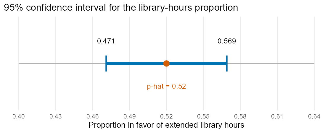
A number line centered at the sample proportion 0.52, with a bracket extending 0.049 in each direction to the endpoints 0.471 and 0.569; the bracket is exactly as wide on the left of the center mark as on the right.

Figure 1. A number line centered at $\hat p = 0.52$ , with a bracket extending 0.049 in each direction to the endpoints 0.471 and 0.569; the bracket is exactly as wide on the left of the center mark as on the right.

3A confidence interval for a mean¶

For a sample mean $\bar x$ from a large sample, the parallel interval is

\bar x \ \pm\ z^\star\dfrac{s}{\sqrt n}

using the sample standard deviation $s$ as a stand-in for the (usually unknown) $\sigma$ — reasonable once $n$ is large.

Worked Example 2 — used textbooks. The bookstore’s buy-back records for $n=45$ used statistics textbooks show a mean resale price of $\bar x = \$63.40$ with $s=\$14.75$ . The standard error is $SE = 14.75/\sqrt{45}\approx\$2.20$ . For 95% confidence, $ME = 1.96(2.20)\approx\$4.31$ , giving

63.40 \ \pm\ 4.31 \quad\Longrightarrow\quad (\$59.09,\ \$67.71)

We are 95% confident the true mean resale price of a used statistics textbook this semester is between $59.09 and $67.71.

4What “95% confident” really means¶

“95% confident” describes the procedure, not this one interval. Before you collect data, there is a 95% chance that the random sample you’re about to draw will produce an interval that captures the true parameter. Once the data are in hand and the interval is calculated — $(0.471,0.569)$ , say — the true proportion either is or is not in that fixed range; there is no randomness left to attach a probability to. The honest phrasing:

“We are 95% confident that the true [parameter] lies between [lower] and [upper]” — meaning: if this sampling procedure were repeated many times, about 95% of the resulting intervals would capture the true parameter.

Two common misinterpretations to avoid.

Not correct: “There is a 95% probability the true proportion is between 47.1% and 56.9%.” The parameter is a fixed (if unknown) number, not a random variable — it does not have a “probability” of falling anywhere.
Not correct: “95% of students’ true opinions fall in this interval.” The interval estimates one population parameter (the overall proportion), not the spread of individual responses.

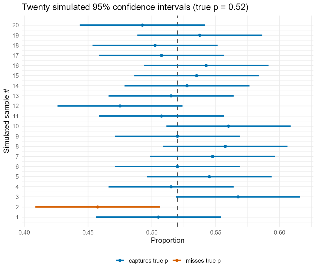
Twenty short horizontal brackets stacked vertically, each a 95% confidence interval built from a different simulated sample drawn from the same population; a dashed vertical line marks the one true parameter value. Nineteen of the twenty brackets cross the dashed line and one does not, illustrating that 95% describes how often the method succeeds across many samples, not the odds attached to any single bracket.

Figure 2. Twenty short horizontal brackets stacked vertically, each one a 95%-confidence interval built from a different simulated sample drawn from the same population; a dashed vertical line marks the one true (known, because simulated) parameter value. About nineteen of the twenty brackets cross the dashed line and about one does not — illustrating that “95%” describes how often the method succeeds across many samples, not the odds attached to any single bracket.

5Confidence level, sample size, and the width of the interval¶

Two knobs control an interval’s width. Raise the confidence level and $z^\star$ grows, widening the interval — a more trustworthy net has to be cast wider. Raise the sample size $n$ and $SE$ shrinks (it has $\sqrt n$ in the denominator), narrowing the interval at a fixed confidence level. Using the textbook-price example:

$n$	$SE$	95% margin of error
45	$2.20	$4.31
90	$1.55	$3.05
180	$1.10	$2.15

Quadrupling $n$ (45 → 180) only cuts the margin of error roughly in half, because $SE$ shrinks with $\sqrt n$ , not with $n$ itself — more data buys precision, but at a diminishing rate.

See it in R.

library(mosaic); library(BSDA)

# Worked Example 1: library-hours poll, phat = 208/400 = 0.52
prop.test(208, 400, conf.level = 0.95, correct = FALSE)$conf.int

# Worked Example 2: used-textbook price, x-bar = 63.40, s = 14.75, n = 45
zsum.test(mean.x = 63.40, sigma.x = 14.75, n.x = 45, conf.level = 0.95)$conf.int

prop.test(208, 400, conf.level = 0.95, correct = FALSE)$conf.int returns $(0.4711,\ 0.5685)$ — R’s Wilson-score method, a slight refinement of the by-hand formula, which for a sample this large agrees with the hand-built $(0.471,\ 0.569)$ to the nearest tenth of a percentage point. zsum.test(mean.x = 63.40, sigma.x = 14.75, n.x = 45, conf.level = 0.95)$conf.int returns $(59.09,\ 67.71)$ , matching the hand calculation exactly, because zsum.test uses the identical $\bar x \pm z^\star\cdot SE$ formula taught this week. Either interval can also be pulled out with confint() on the saved test object instead of $conf.int.

6Check your understanding¶

A poll of $n=250$ registered voters finds 135 in favor of a ballot measure. Compute $\hat p$ , then build a 95% confidence interval ( $z^\star=1.96$ ). State the margin of error.
Using the library-hours poll ( $\hat p=0.52$ , $n=400$ ), build a 90% confidence interval instead of the 95% interval from the example. Is it narrower or wider? Why?
A random sample of $n=36$ campus coffee-shop receipts has $\bar x = \$6.10$ and $s=\$2.40$ . Construct a 95% confidence interval for the true mean receipt total.
Explain in your own words why quadrupling the sample size only cuts the margin of error in half, rather than in fourth.
A student says, “There’s a 95% probability the true proportion favoring extended library hours is between 47.1% and 56.9%.” What is wrong with this statement, and what is the correct interpretation?
Using the used-textbook example ( $\bar x=\$63.40$ , $s=\$14.75$ , $n=45$ ), build a 99% confidence interval. Is its margin of error larger or smaller than the 95% interval from the example? Why?

7Key terms¶

Confidence interval — a range of plausible values for a population parameter, built as point estimate ± margin of error.
Confidence level — the long-run success rate of the interval-building procedure (e.g., 95% means about 95% of intervals built this way, across repeated samples, capture the true parameter).
Margin of error (ME) — the distance the interval reaches in either direction from the point estimate; $ME = z^\star \cdot SE$ for a large sample.
Critical value $z^\star$ — the number of standard errors needed on each side of the point estimate to reach the stated confidence level (1.645 for 90%, 1.960 for 95%, 2.576 for 99%).