This week in a line: you’ll learn to test whether one specific claimed value is believable, using a test statistic, a p-value, and a clear decide / fail-to-reject rule.
Last week you built a confidence interval — a whole range of plausible values for an unknown population parameter. This week flips the question around. Instead of “what range of values is plausible?” you’ll ask something sharper: “is this one specific claimed value believable, given what my sample shows?” Your roommate insists the coin from the laundry room “seems unfair” — like it lands heads more often than tails. You can’t interrogate a coin, so you flip it, count, and reason from the data. Spelled out formally, that reasoning process is a hypothesis test, and it’s the backbone of almost every “does this actually work?” claim you’ll meet after this course — in a lab report, a business memo, or a news headline.
1Two competing claims: and 
Every hypothesis test starts with two claims about a population parameter that can’t both be true. One is the null hypothesis, — a skeptical, “nothing new going on” claim, always stated as an equality. The other is the alternative hypothesis, — what you suspect might be true instead, stated with , , or . The logic mirrors a courtroom: you assume (innocence) unless the sample data gives strong enough evidence to abandon it.
If uses , the test is two-sided (evidence in either direction counts against ). If uses or , the test is one-sided (only evidence in the stated direction counts).
Coin fairness. No reason to suspect a particular direction, so this is two-sided:
Study-skills workshop. The workshop is designed to raise scores, so this is one-sided:
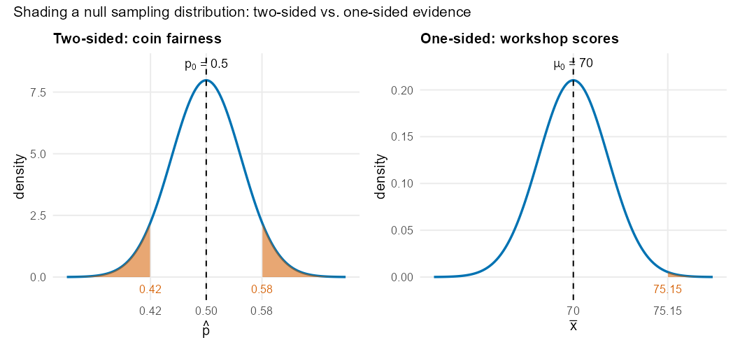
Figure 1. Two bell-shaped sampling-distribution sketches side by side. The left one, centered at , has both tails shaded past a marked point on either side (two-sided evidence). The right one, centered at , has only its right tail shaded past a marked point (one-sided evidence).
2The test statistic: how far from , in SE units
Once you assume is true, ask: how surprising is the sample statistic under that assumption? The test statistic answers this the same way Week 6’s z-score did — by measuring distance in standard error units, using the standard errors you built in Weeks 9–10:
Here and are the sample statistic actually observed; and are the hypothesized values from ; and is the standard error computed as if were true. A large means the sample landed far from what predicted — evidence against it.
3The p-value: probability of data this extreme, if is true
The p-value is the probability of getting a test statistic at least as extreme as the one you observed, assuming is true. It is a conditional probability — conditioned on an assumption you haven’t confirmed.
The decision rule compares the p-value to a significance level — the risk of a wrong rejection you agree to accept before seeing the data, usually in this course:
| Rule | Decision | Meaning |
|---|---|---|
| p-value | Reject | statistically significant evidence for |
| p-value | Fail to reject | not enough evidence to abandon |
Failing to reject is not the same as proving true. It only means the sample didn’t give strong enough evidence to abandon it — absence of evidence isn’t evidence of absence.
Worked Example 1 — Is the laundry-room coin fair? Simulating flips of a genuinely fair
coin (, set.seed(1209)) gives 42 heads, so . Under ,
The sample proportion sits 1.60 SEs below the hypothesized 0.5. For a two-sided test, the p-value adds both tails beyond : . Since , we fail to reject : this sample of 100 flips does not give strong evidence the coin is unfair. (It might still be biased — 100 flips just wasn’t enough to tell. More on that below.)
4One-sided tests, and the cost of being wrong
Worked Example 2 — Does the study-skills workshop raise scores? CSUB’s math-placement diagnostic
(a computer-adaptive exam scored on a 0–200 scale) has historically averaged points with a
known population standard deviation (a stated benchmark built from many prior years, so
is treated as known here — the large-sample z story). This term, students completed a
new study-skills workshop before testing; simulating their scores (set.seed(1209), centered 4 points
above the historical mean to model a real but modest effect) gives and a sample spread
. Since is treated as known, the test still uses , not , in the standard
error (Week 14’s t-test will use instead):
is one-sided, so the p-value is only the right tail beyond : . Since , we reject : this sample gives strong evidence the workshop group’s average diagnostic score is higher than the historical 70.
Statistical significance vs. practical importance. The average shift (about 5 points) is statistically clear, but the spread among individual students, , is nearly three times that shift — a large n makes small average effects easy to detect statistically, but a program director still has to ask separately whether a 5-point average bump is worth the workshop’s cost and time across students who vary that much individually.
Type I and Type II errors. No decision rule is ever certain, because you never actually know whether is true. A Type I error is rejecting an that is actually true; by design, this happens with probability exactly . In Example 2, if the workshop truly had no effect, a batch of 40 students would still produce a “significant” result about 5% of the time purely by chance — the price of using . A Type II error is failing to reject an that is actually false. In Example 1, if the laundry-room coin actually is slightly biased, 100 flips may simply not be enough evidence to catch it — we’d fail to reject fairness even though it’s false. Which error costs more depends on context: a factory that stops a good production line (Type I) wastes time and money; a factory that lets a broken line keep running (Type II) ships defective product.
See it in R.
library(mosaic)
library(BSDA)

# Worked Example 1: coin fairness, two-sided --------------------------------
set.seed(1209)
flips <- rflip(100, prob = 0.5)          # 42 heads out of 100 this run
prop.test(x = 42, n = 100, p = 0.5, alternative = "two.sided", correct = FALSE)

# Worked Example 2: workshop diagnostic scores, one-sided --------------------
zsum.test(mean.x = 75.15, sigma.x = 12, n.x = 40, mu = 70, alternative = "greater")
prop.test prints X-squared = 2.56, p-value = 0.1096 — note , the same computed
by hand. zsum.test prints z = 2.7143, p-value = 0.003321, matching Example 2 above.
5Check your understanding
A campus dining hall claims “at least 90% of students are satisfied with the new menu.” A student group suspects satisfaction is actually lower and surveys a random sample to test this. State and in symbols, and say whether the test is one-sided or two-sided.
Explain in your own words why “fail to reject ” is not the same as “ is true.” Use the coin-fairness result from Worked Example 1 in your explanation.
A classmate looks at Worked Example 2’s result (, ) and says, “That means there’s only a 0.33% chance the workshop doesn’t work.” Explain what is wrong with that statement, and give the correct interpretation of the p-value.
Using the coin-fairness setup from Worked Example 1 (, , same ), suppose the sample had instead come out . Compute the z test statistic.
A researcher sets in advance and gets a p-value of 0.04. Should they reject or fail to reject ? Now suppose they had set instead, for that same p-value — does the decision change? What does this tell you about the role of ?
In one or two sentences, describe a real (non-classroom) situation where a Type I error and a Type II error would have different real-world costs — for example, a medical test, a spam filter, or a quality-control check. Name which error is more costly in your example and why.
6Key terms
Null hypothesis, — the skeptical, “nothing new going on” claim about a parameter, always stated as an equality; assumed true unless the data give strong evidence otherwise.
Alternative hypothesis, — the claim you suspect might be true instead, stated with , , or .
One-sided / two-sided test — a test where points in one direction ( or ) vs. either direction ().
Test statistic — a standardized measure (here, ) of how far the sample statistic is from the value claims, in standard-error units.
p-value — the probability of a test statistic at least this extreme, assuming is true.
Significance level, — the pre-chosen risk of a wrong rejection; commonly 0.05.
Statistically significant — the decision reached when the p-value is less than .
Type I error — rejecting a true ; occurs with probability by design.
Type II error — failing to reject a false .