1A range, not a guess
Every spring, the Bakersfield Californian runs a story about the oil patch:
hiring is up, hiring is down, a rig count moved. Underneath those headlines is a
real number the Bureau of Labor Statistics publishes for the Bakersfield metro
area — Mining & Logging payroll employment, which in Kern County is almost
entirely the oilfield workforce. Over the ten years 2015–2024 it averaged about
8.6 thousand jobs per year (kern_energy_employment, variable
ces_mining_logging_thsd).
But “8.6 thousand” is the average of just ten yearly numbers, and those ten years are themselves a sample of the larger process that generates oilfield employment. If the decade had played out a little differently — a different oil price here, a different drilling decision there — the average would have landed somewhere else. So a single number, by itself, hides the question a decision-maker actually cares about: how far off could it be?
A confidence interval answers exactly that. Instead of reporting one number,
you report a range of plausible values, together with how confident you are
that the range captures the truth. For these ten years, the 95% confidence
interval for the mean annual oilfield payroll runs from about 7.70 to 9.52
thousand jobs — a number we will compute from scratch, and learn to read
correctly, in this chapter. (All figures here are derived from the real
kern_energy_employment dataset; see its
codebook.)
2Learning objectives
By the end of this chapter you will be able to:
Interpret a confidence interval correctly — and recognize the common misinterpretations that even textbooks sometimes slip into.
Construct a confidence interval for a mean or a proportion using the CLT-based formula .
Construct a bootstrap confidence interval by resampling in R, and compare it to the formula-based interval.
Explain how the confidence level and the sample size change the width of an interval.
Report an interval estimate with its margin of error in plain language for a decision-maker who has never taken a statistics class.
This chapter builds directly on the sampling distribution from Chapter 6: the pattern of how a sample statistic varies from one sample to the next. A confidence interval is that idea put to work. Before going on, make sure you are comfortable with the standard error () — the spread of a sampling distribution — which we will lean on in every section.
37.1 What a confidence interval is
3.1Intuition
In Chapter 6 you learned that a sample statistic — say the sample mean — bounces around from sample to sample, and that the spread of that bouncing is the standard error (). The Central Limit Theorem told you the bouncing is approximately Normal and centered on the true parameter.
Turn that idea around. If usually lands within about two standard errors of the truth, then the truth is usually within about two standard errors of . So we can take our one observed estimate and reach out a couple of standard errors in each direction:
That reach-out interval is a confidence interval: a range of plausible values for the unknown parameter. The “a few” is a critical value chosen so that the interval is wide enough to capture the truth a stated percentage of the time — the confidence level.
3.2The correct interpretation (read this twice)
A 95% confidence interval does not mean “there is a 95% probability the parameter is in this interval.” Once you have computed an interval like , the true mean either is or isn’t inside it — there is no probability left to assign. The 95% describes the procedure, across many hypothetical samples:
If we repeated the whole study many times and built a 95% interval each time, about 95% of those intervals would contain the true parameter.
The confidence is in the method, not in any single interval. We unpack this with a simulation in Section 6, and we drill the right and wrong phrasings in Worked Example 4.
3.3Formula
For a population mean , when the population standard deviation is unknown (the realistic case), the interval is
Defining every symbol the first time it appears:
(“x-bar”) — the sample mean, our point estimate of .
(“mu”) — the unknown population mean we are estimating.
— the sample standard deviation (how spread out the data are).
— the sample size (number of observations).
— the standard error of the mean: how much varies from sample to sample.
— the critical value from the -distribution with degrees of freedom; the multiplier that makes the interval wide enough for the chosen confidence level.
The two pieces after the ± together, , are the margin of error (ME) — the “±” reach of the interval.
For a population proportion , the parallel formula uses a critical value from the Normal distribution and the proportion’s standard error:
where (“p-hat”) is the sample proportion estimating the population proportion .
3.4In R
In the mosaic/BSDA stack, the one-sample interval comes straight from base R’s
t.test(), written with the formula ~ variable (read the ~ as “just this
variable”). The line you want in the printout is 95 percent confidence interval.
energy <- read.csv("data/processed/kern_energy_employment.csv")

# 95% CI for the mean annual oilfield (Mining & Logging) payroll, in 1000s jobs.
# t.test also runs a test against a default mu = 0 (the "t = ..., p-value = ..."
# line); we are only ESTIMATING here, so ignore that line and read the
# "95 percent confidence interval" block.
ci_oil <- t.test(~ ces_mining_logging_thsd, data = energy, conf.level = 0.95)
ci_oil
The printout is a compact block: a test line (t = 21.43, df = 9, p-value = 4.9e-09), then the 95 percent confidence interval — here
7.701093 9.518907 — and finally the sample estimates line giving
mean of x . We ignore the test line (its null “the mean is 0” is not
a question anyone asks about a payroll count) and read the interval.
# The test object carries the computed pieces for reuse:
ci_oil$estimate    # x-bar (the sample mean)
ci_oil$stderr      # the standard error, s / sqrt(n)
ci_oil$conf.int    # the 95% interval (lower, upper)
The interval is thousand jobs — the number from
Section 1, now derived — with and .
Every digit in this paragraph came from kern_energy_employment, not from
hand-waving.
47.2 The margin of error, the level, and the sample size
4.1Intuition
The margin of error has only two moving parts, and each one is intuitive:
Confidence level critical value. Want to be more confident the interval catches the truth? You must cast a wider net, so (or ) grows. A 99% interval is wider than a 95% interval, which is wider than a 90% interval — for the same data.
Sample size standard error. More data makes steadier, so shrinks. Because of the , cutting the margin in half takes four times the data, not twice.
There is a genuine trade-off here: a wider interval is more likely to be right but less useful (it says less); a narrower interval is more informative but riskier. Choosing a confidence level is choosing where to sit on that trade-off.
4.2Formula
For a mean, the margin of error is
If you are planning a study and want the margin no larger than some target (using a planning value for the spread and the Normal ), solve Equation for . Set the margin equal to the target and unwind it one step at a time: from , multiply both sides by and divide by to get , then square both sides:
Always round up to the next whole observation.
4.3In R
We can show the level effect directly on the Kern data by asking t.test() for
three confidence levels and reading off the widths.
levels <- c(0.90, 0.95, 0.99)
# For one confidence level, pull t.test's interval and record its width;
# sapply runs that same recipe for each of the three levels and collects them.
widths <- sapply(levels, function(cl) {
  ci <- t.test(~ ces_mining_logging_thsd, data = energy,
               conf.level = cl)$conf.int
  diff(ci)                       # upper - lower = interval width
})
data.frame(level = levels, width_thousands = round(widths, 3))
The widths grow with the level — from about 1.47 (90%) to 2.61 thousand jobs (99%) on these same ten years. The 90% interval is the narrowest because it demands the least confidence.
57.3 Confidence intervals without a formula: the bootstrap
5.1Intuition
The formula in Equation leans on the CLT and on the -distribution being a good description of how varies. When the sample is small or oddly shaped, you might wonder whether that description holds. The bootstrap sets the formula aside and lets the data describe their own variability.
The trick is almost cheeky: treat your sample as if it were the population, then draw new samples from your sample, with replacement, each the same size . Each such resample gives a new . Do it thousands of times and you have rebuilt a sampling distribution — empirically, with no formula. The middle 95% of those resampled means is a 95% bootstrap confidence interval (the percentile method).
5.2Formula
There is no closed-form formula; the procedure is the definition. For resamples:
Resample values from the data with replacement; compute the statistic. We write a resampled mean as — the star marks it as coming from a resample rather than the original data, and counts which resample it is.
Repeat for , where is the number of resamples (say ).
The percentile interval is the range between the 2.5th and 97.5th percentiles of the resampled statistics — the middle 95% of them.
5.3In R
oil <- energy$ces_mining_logging_thsd
n   <- length(oil)

set.seed(2200)                       # reproducible resampling
B <- 10000
boot_means <- replicate(B, {
  resample <- sample(oil, size = n, replace = TRUE)
  mean(resample)
})

boot_ci <- quantile(boot_means, c(0.025, 0.975))
round(boot_ci, 3)
The bootstrap interval lands close to the formula interval , but it is a touch narrower: its dashed bounds sit near , so its lower end is about two tenths of a thousand jobs above the formula’s 7.70. That gap is expected — the percentile bootstrap does not carry the -distribution’s small-sample tail-widening, and with only years that widening is not negligible. The near-agreement is still the lesson: when conditions hold, the formula and the bootstrap tell essentially the same story, which is exactly why we trust the convenient formula. When they disagree sharply, the bootstrap is the warning light.
ggplot(data.frame(boot_means = boot_means), aes(x = boot_means)) +
  geom_histogram(bins = 40, fill = okabe_ito[1], colour = "white") +
  geom_vline(xintercept = boot_ci, linetype = "dashed",
             colour = okabe_ito[4], linewidth = 0.9) +
  labs(
    x = "Resampled mean oilfield payroll (thousands of jobs)",
    y = "Number of resamples",
    title = "Bootstrap sampling distribution (B = 10,000)"
  ) +
  theme_minimal(base_size = 12)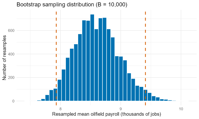
Bootstrap distribution of the mean annual oilfield payroll.
67.4 Why “95% confident” means what it means
6.1Intuition
The single most-tested idea in this chapter is the interpretation from Section 3. The cleanest way to see it is to play God: invent a population whose true mean we know, draw many samples, build a 95% interval from each, and count how many capture the truth. It should be about 95%.
6.2In R
We use a population mean of 8.61 (our oilfield estimate) just to have a concrete target; the point is the counting, not the number.
set.seed(2200)
true_mu    <- 8.61
# Round-number PLANNING value for the made-up population, not the sample
# statistic. We deliberately use 1.27 (not the sample s = 1.271) because this
# is an invented "true" population we draw from — the point is the counting,
# not matching the Kern data exactly.
true_sigma <- 1.27
n_each     <- 10
n_studies  <- 1000

captured <- replicate(n_studies, {
  samp <- rnorm(n_each, mean = true_mu, sd = true_sigma)  # 10 fake draws from a bell curve
  ci   <- t.test(samp, conf.level = 0.95)$conf.int        # build a 95% CI
  ci[1] <= true_mu && true_mu <= ci[2]                    # did this one catch mu?
})

mean(captured)   # share of the 1000 intervals that captured the truth
Run this and you will get a number close to 0.95 — about 95% of the
intervals contain the true mean, exactly as advertised. (Each interval either
catches or not, a TRUE/FALSE; mean() of TRUE/FALSE values is just
the fraction that were TRUE.) The 5% that miss are not mistakes in arithmetic;
they are the price of the method, baked into the word “95%.”
The simulator below lets you see that counting happen. Each row is one 95% interval built from a fresh sample; press Play and watch batch after batch of twenty intervals, a stubborn handful missing the target every time.
Figure 1:Confidence-interval coverage (simulated) — press Play: each batch draws twenty fresh 95% intervals; the vermillion ✕ intervals are the ~5% that miss the true mean (green dashed line), while the blue-circle intervals capture it.
Going deeper (optional) — why a CI and a two-sided test agree
This box is enrichment; you can skip it without missing any required skill.
There is a clean duality between a confidence interval and a hypothesis test (Chapter 8). A 95% confidence interval is exactly the set of “null” values that a two-sided test at significance level would not reject. So the two tools are the same evidence wearing different clothes:
If a value sits inside the 95% interval, a two-sided test of would fail to reject at — the data are consistent with that value.
If sits outside the interval, the same test would reject it.
That is why Section 7.3’s interval “including 0.50” is the same statement as “a two-sided test would not reject .” The interval does more than the test, though: it hands you the whole range of values the data cannot rule out, not just a yes/no verdict about one of them. We make this duality precise in Chapter 8; here it is enough to notice that “is in the interval?” and “would a test reject ?” are two ways of asking one question.
7Worked examples
Every worked example below follows the same five steps, so you always know what comes next:
State the estimate — the sample mean or sample proportion you are reaching out from.
Find the standard error — how much that estimate wobbles from sample to sample.
Pick the critical value — (means) or (proportions) for your confidence level.
Build the margin of error , and form the interval .
Say it in plain words — what the interval means for a real reader.
7.1Worked Example 1 — Mean oilfield payroll (the Kern hook)
Question. Using all ten years of kern_energy_employment, build and
interpret a 95% confidence interval for the mean annual oilfield (Mining &
Logging) payroll in the Bakersfield MSA.
Intuition. We have one sample of yearly averages. The sample mean is our best single guess; the interval reaches out a couple of standard errors on each side to express how uncertain that guess is.
Formula. Mean interval, Equation: , with .
Computation. From the data, , , , so . The 95% critical value is , giving .
t.test(~ ces_mining_logging_thsd, data = energy, conf.level = 0.95)$conf.intSo the interval is thousand jobs.
Interpretation. We are 95% confident that the mean annual oilfield payroll for the Bakersfield MSA over this period lies between about 7,700 and 9,500 jobs. The interval does not tell us where any single year fell (2015 was 11.4k, well above it); it estimates the average level and how precisely ten years pin it down.
7.2Worked Example 2 — Total nonfarm payroll, three confidence levels
Question. For the same dataset’s total nonfarm payroll
(ces_total_nonfarm_thsd, thousands of jobs), construct 90%, 95%, and 99%
confidence intervals for the mean and compare their widths.
Intuition. Same data, three different “nets.” More confidence wider net.
Formula. Equation with equal to 1.833 (90%), 2.262 (95%), and 3.250 (99%).
Computation. Here , , , so .
for (cl in c(0.90, 0.95, 0.99)) {
  ci <- t.test(~ ces_total_nonfarm_thsd, data = energy, conf.level = cl)$conf.int
  cat(sprintf("%.0f%% CI: (%.1f, %.1f)  width = %.1f\n",
              100 * cl, ci[1], ci[2], diff(ci)))
}
This prints the 95% interval as thousand jobs, with the 90% interval narrower and the 99% interval wider.
Interpretation. All three intervals are centered on the same estimate (271.7k jobs); confidence buys width. A planner who needs to be very sure quotes the 99% range; one who wants a tighter working estimate accepts the 90% range and its higher chance of missing.
7.3Worked Example 3 — A proportion: high-burden tracts
Question. In kern_calenviroscreen, a census tract is “high-burden” if its
statewide CalEnviroScreen percentile is at least 75. Of the Kern tracts with a
score, what fraction are high-burden, and what is a 95% confidence interval for
that proportion?
Intuition. We have a yes/no label per tract; is the observed fraction, and we reach out standard errors to estimate the population proportion .
Formula. Proportion interval, Equation: , with for 95%. First check the success–failure condition: and .
Computation.
ces  <- read.csv("data/processed/kern_calenviroscreen.csv")
high <- ifelse(ces$ces_percentile >= 75, "high_burden", "not")  # label tracts
x <- sum(high == "high_burden", na.rm = TRUE)   # 73 high-burden tracts
n <- sum(!is.na(high))                           # 147 scored tracts
# prop.test returns a Wilson (score) interval; correct = FALSE drops the
# continuity correction so it lines up with the by-hand Wald interval below.
prop.test(x, n, correct = FALSE)$conf.int
Here 73 of 147 scored tracts are high-burden, so ,
, and
. The success–failure check passes easily
(, , both ). The by-hand Wald interval is
; prop.test() prints the Wilson score
interval , which for and near one-half agrees
with the Wald interval to within about a thousandth.
Interpretation. We are 95% confident that between about 42% and 58% of Kern’s scored tracts rank in the worst statewide quarter for environmental burden. The interval comfortably includes 50%, so these data are consistent with “about half” — a sobering headline that the margin of error keeps honest.
7.4Worked Example 4 — Saying it right (interpretation drill)
Question. A student reports the Worked Example 1 interval four ways. Mark each as correct or incorrect, and fix the wrong ones.
| # | Statement | Verdict |
|---|---|---|
| a | “There is a 95% probability the true mean is between 7.70 and 9.52.” | ❌ |
| b | “95% of years had oilfield payroll between 7.70 and 9.52 thousand.” | ❌ |
| c | “If we repeated this study many times, about 95% of the intervals we’d build would contain the true mean.” | ✅ |
| d | “We are 95% confident the true mean oilfield payroll is between 7.70 and 9.52 thousand jobs.” | ✅ |
Reasoning.
(a) treats this fixed interval as having a probability. Once computed, the interval either contains or not; the 95% describes the procedure, not this instance. Fix: use (c) or (d)'s wording.
(b) confuses a confidence interval for the mean with a range for individual years. Indeed 2015’s value (11.4k) lies outside it. A range for individual values is a prediction interval, a different and wider thing.
(c) is the textbook-correct frequency statement.
(d) is the accepted plain-language shorthand: “confident,” not “probability.”
Interpretation. The difference between (a) and (d) looks like hair-splitting but is the whole idea of the chapter: confidence lives in the method that generates intervals, not in any single interval you happen to hold.
8Try it
Put these ideas in motion with the two companion tools built for this chapter:
Shiny — Statistics Explorer, “CI Calculator & Visualizer” module. Pick a dataset, choose a variable and a confidence level, and watch the interval (and the exact R code that produced it) update live. Launch the app with
shiny::runApp("shiny-explorer")and open the Confidence Intervals tab. The code panel uses the samet.test()/prop.test()calls you see above, so the app and this book teach identical syntax.Jupyter lab —
labs/lab07-confidence-intervals.ipynb. A guided, R-kernel notebook: rebuild the oilfield interval, run your own bootstrap, and write the coverage-simulation loop from Section 6. Starter code and a reflection prompt are included; the instructor solution is ininstructor/lab-solutions/.
9Chapter summary
A confidence interval reports a range of plausible values for an unknown parameter, in the form , instead of a single guess.
For a mean: with . For a proportion: , after the success–failure check.
The margin of error has two levers: a higher confidence level widens it; a larger sample size narrows it, but only at the rate .
The bootstrap rebuilds the sampling distribution by resampling the data with replacement; its percentile interval agrees with the formula when conditions hold and warns you when they don’t.
“95% confident” is a statement about the procedure: about 95% of intervals built this way capture the truth. It is not a probability about one fixed interval, nor a range for individual observations.
On the real Kern oil data, the 95% interval for mean annual oilfield payroll is thousand jobs — a result we computed, never assumed.
10FAQ
Q1. Why do we add and subtract the margin of error instead of just reporting the sample mean? Because the sample mean would be wrong to some unknown degree. The margin of error is an honest admission of how far off it could plausibly be; dropping it pretends to a precision the data don’t have.
Q2. Is a 99% interval “better” than a 95% interval? Not better — more cautious. It is more likely to contain the truth but says less because it is wider. The right level depends on how costly a miss would be for your decision. 95% is a common default, not a law.
Q3. My bootstrap interval changed slightly when I ran it again. Did I make a
mistake?
No — resampling uses random draws, so two runs differ a little. Set a seed
(set.seed(2200)) for reproducibility, and increase (the number of
resamples) to make the wobble smaller.
Q4. When should I use and when ? Use (with ) for a mean, because we estimate the spread from the data. Use for a proportion. With large the two critical values nearly coincide, but in this course we keep the distinction explicit.
Q5. The interval includes a “no-difference” value like 0 (or 50%). So what? That is informative: if a plausible-values range includes the boundary that means “no effect,” your data are consistent with no effect. This is the bridge to hypothesis testing in Chapter 8 — a 95% interval that excludes the null value corresponds to a significant test at .
Q6. Does a wider sample range (more spread) make the interval wider? Yes. The margin of error contains in the numerator, so a more variable variable produces a wider interval — more spread means more uncertainty about the mean, all else equal.
Q7. How big a sample do I need for a margin of error I can live with? Solve Equation: , using a planning value for the spread and your target margin . Always round up. Halving the margin quadruples the required .
Q8. Can I build a confidence interval from summary statistics if I don’t have
the raw data?
Yes. BSDA’s tsum.test(mean.x = 8.61, s.x = 1.271, n.x = 10) builds the mean
interval from summaries alone — handy when a report gives you , , and
but not the data.
11Practice problems
Conceptual & interpretation
In one sentence, explain why a confidence interval is more honest than reporting only a sample mean.
State, in plain language, the correct interpretation of a 95% confidence interval. Then write one incorrect interpretation and say what is wrong with it.
True or false, with a reason: “A 90% confidence interval is wider than a 99% confidence interval built from the same data.”
Explain why the bootstrap interval and the formula interval usually agree, and name one situation in which they might not.
A poll reports “52% ± 4 percentage points.” Identify the point estimate, the margin of error, and the implied confidence interval.
Why does quadrupling the sample size only halve the margin of error?
Computation — means
A sample has , , . Construct a 95% confidence interval for . (Use .)
Using
kern_energy_employment, the Kern County unemployment rate (kern_unemp_rate) over 2015–2024 has , , . Build a 95% confidence interval for the mean unemployment rate.For the same unemployment-rate data, build a 90% interval (use ) and a 99% interval (use ). Which is widest, and why?
A sample of commute times has minutes and minutes. Construct a 95% interval for the mean commute time (use ).
Re-express the oilfield-payroll 95% interval thousand jobs in the form . What are and ?
A study reports a 95% confidence interval for a mean as . What were the sample mean and the margin of error?
Computation — proportions
In a sample of households, have rooftop solar. Check the success–failure condition and build a 95% interval for .
Of Kern tracts surveyed, report a particular hazard. Estimate and give a 95% confidence interval.
For the high-burden-tract example (Section 7.3), the 95% interval was . Does it include 0.50? What does that tell you?
A 95% interval for a proportion is . State the interval and explain whether the value 0.25 is plausible for .
Sample-size planning & level effects
You want a 95% confidence interval for a mean with margin of error no larger than , and a planning value . Use Equation to find the minimum sample size.
Repeat problem 17 with the same but a tighter target . Compare your answer to problem 17 and comment on the cost of precision.
For a 95% interval estimating a proportion to within , using the conservative planning value , find the minimum ().
Explain, using Equation, two different changes you could make to a study to narrow a confidence interval, and a cost of each.
Data-driven & R
Write the R call (mosaic
t.testwith the~ variableformula) that produces a 90% confidence interval for the mean total nonfarm payroll (ces_total_nonfarm_thsd) fromkern_energy_employment.Describe, in steps (no code required), how you would build a bootstrap 95% interval for the mean unemployment rate from
kern_energy_employment.The coverage simulation in Section 6 returned about 0.95. If you changed the confidence level in that loop to 0.80, what proportion of intervals would you expect to capture the truth, and would the intervals be wider or narrower?
Using
kern_energy_employment, the 95% interval for mean oilfield payroll is . A reporter writes, “95% of years had oilfield payroll in this range.” Explain why that is wrong and write a correct one-sentence summary.A colleague gives you only , , and for oilfield payroll (no raw data). Write the
tsum.test()call (BSDA) using its summary-statistics arguments (mean.x,s.x,n.x) and state the 95% interval you expect.
12Glossary additions
New terms introduced in this chapter are defined in the
glossary appendix: confidence interval,
confidence level, margin of error, critical value, bootstrap, and
coverage. The per-chapter glossary fragment lives at book/ch07/_glossary.md.
13Resumen en español
Resumen del capítulo
En este capítulo aprendiste a construir e interpretar un intervalo de confianza (confidence interval): un rango de valores plausibles para un parámetro poblacional desconocido. En lugar de reportar un solo número, el intervalo te dice con cuánta certeza puede equivocarse esa estimación puntual.
El ejemplo central del capítulo proviene de datos reales del condado de Kern: el empleo anual en la industria petrolera de la zona metropolitana de Bakersfield, registrado en el conjunto de datos kern_energy_employment. A partir de diez años de datos, la media muestral (sample mean) fue de aproximadamente 8.61 miles de empleos, y el intervalo de confianza (confidence interval) del 95% resultó ser de 7.70 a 9.52 miles de empleos.
La fórmula general es:
estimación ± (valor crítico) × error estándar
Para la media, el error estándar (standard error) es , y el valor crítico (critical value) proviene de la distribución con grados de libertad (degrees of freedom). Para una proporción, se usa la distribución normal con .
Dos palancas controlan el ancho del intervalo: aumentar el nivel de confianza (confidence level) lo hace más amplio; aumentar el tamaño de muestra (sample size) lo estrecha, pero solo a razón de , lo cual significa que para reducir el margen de error (margin of error) a la mitad se necesita cuadruplicar .
El capítulo también presentó el bootstrap (bootstrap): un método de remuestreo que reconstruye la distribución muestral sin fórmulas. Con los datos del petróleo de Kern, el intervalo bootstrap coincidió muy de cerca con el intervalo de fórmula, lo que confirma que ambos enfoques cuentan la misma historia cuando las condiciones se cumplen.
La interpretación correcta es crucial: decir “estamos 95% seguros de que la media verdadera está entre 7.70 y 9.52 miles de empleos” es aceptable. Decir “hay un 95% de probabilidad de que la media verdadera esté en este intervalo exacto” es incorrecto: el 95% describe el procedimiento (procedure), no este intervalo en particular.
En R, la función t.test() (con la fórmula ~ variable, a partir de datos crudos) o tsum.test() del paquete BSDA (a partir de resúmenes) construye el intervalo; se lee el bloque 95 percent confidence interval de la salida.