1The opening question
A campus wellness program runs an experiment. It recruits 200 students, randomly assigns 100 to a treatment group (an 8-week activity-coaching program) and 100 to a control group (no coaching), and at the end records each student’s average daily active minutes from a wearable tracker. The treatment group averaged more active minutes than the control group. The program director is thrilled — until a skeptical colleague asks the only question that matters:
“Random assignment splits people into two piles. Even if coaching did nothing at all, one pile will almost always come out a little ahead just by luck. How do you know your difference isn’t just that luck?”
That single question is the whole of this chapter. Let us put a number on it.
# Load the randomized two-group experiment (a *simulated* classroom dataset,
# committed with its generator; see the codebook). 200 students, 100 per arm.
fit <- read.csv("data/processed/fitness_tracker_sim.csv")

# Mean daily active minutes, "broken down BY group": that is what the mosaic
# formula active_minutes ~ group means -- read "~" as "by". It returns one mean
# per group, labeled with the group name.
grp_means <- mean(active_minutes ~ group, data = fit)
grp_means

# The observed difference: treatment mean minus control mean.
obs_diff <- unname(grp_means["treatment"] - grp_means["control"])
round(obs_diff, 3)
The treatment group averaged about 36.87 active minutes per day; the control group about 27.94. The observed difference is
So the program did produce a 8.92-minute gap. The skeptic’s question is whether a gap that big could plausibly appear even if coaching changes nothing. By the end of this chapter you will answer it with a number — and you will know exactly what that number does, and does not, mean.
2Learning objectives
By the end of this chapter you will be able to:
State null and alternative hypotheses for a research question, and define the significance level , a Type I error, and a Type II error.
Run a randomization (permutation) test in R and use the simulated null distribution to find a p-value.
Interpret a p-value correctly, and connect a test decision to the corresponding confidence interval.
Evaluate the difference between statistical and practical significance, and the role sample size plays in each.
Identify the conditions a test requires and the consequences of violating them.
This chapter expands ISRS sections 2.1–2.3 (randomization case studies and hypothesis testing). It assumes you have met sampling distributions and the CLT (Chapter 6) and confidence intervals (Chapter 7).
31. Hypotheses: the two competing stories
3.1Intuition
Every hypothesis test is a contest between two stories about how the data were produced.
The null story is the boring one: nothing is going on. Coaching has no effect; any difference between the groups is just the luck of the random split. This is the skeptic’s position, and — crucially — we assume it is true while we weigh the evidence, the way a court assumes a defendant innocent until the evidence says otherwise.
The alternative story is the interesting one: something is going on. Coaching really does change active minutes, so the groups differ for a real reason, not just chance.
The test never tries to prove the alternative directly. Instead it asks: if the null story were true, how surprising would our data be? If the data would be very surprising under the null story, we abandon it in favor of the alternative. If the data are unremarkable under the null story, we have no grounds to abandon it. That asymmetry — we can reject the null but never prove it — is the engine of the whole method.
3.2Formula (notation)
We write the two stories as the null hypothesis and the alternative hypothesis . For our two-group experiment they concern the difference in population mean active minutes, :
Defining every symbol the first time it appears:
(“mu-treatment”) — the population mean daily active minutes if everyone like our subjects received coaching. A fixed, unknown number (a parameter).
(“mu-control”) — the population mean if no one received coaching.
(“H-naught”) — the null hypothesis: the two population means are equal, so their difference is 0.
(“H-A”) — the alternative hypothesis: the means differ. The makes this a two-sided alternative (we would care about a difference in either direction). If theory predicted a direction in advance we could use a one-sided alternative, .
Two rules that are easy to forget and costly to break:
Hypotheses are always about parameters — fixed, unknown population numbers like a population mean or a population proportion — never about statistics, the numbers we compute from a sample like a sample mean (“x-bar”) or a sample proportion (“p-hat”). We already know $\bar{x}_{\text{trt}}
\bar{x}_{\text{ctrl}} = 8.92\mu$'s.
The hypotheses are chosen before looking at the data — or at least independently of the particular result we got — so we are not just drawing a target around wherever the arrow landed.
3.3In R
In this book we will do most of the testing by simulation (Section 2), but it
is worth seeing the group summaries that the hypotheses are about. In the mosaic
stack, favstats() gives a full teaching summary of a variable broken down by
group — again the y ~ group (“y by group”) formula:
# favstats() summarizes active_minutes separately for each group: it prints
# min, Q1, median, Q3, max, the mean, the sd, the count n, and any missing.
favstats(active_minutes ~ group, data = fit)
Read the mean, sd, and n columns: and
are the two sample means (your best single-number
summary of each group), and are the two
sample standard deviations (how spread out each group is), and is the
number of students in each group. The treatment group
(, , )
sits above the control group (,
, ). says those two population
means are really equal; says they are not. Now we test.
42. The randomization test: chance, made visible
4.1Intuition
Here is the beautiful idea at the heart of this chapter. The students were assigned to groups by a coin flip we controlled. So we can re-run that coin flip on a computer.
If the null story is true — coaching does nothing — then each student’s active minutes were going to be whatever they were going to be, regardless of which group label they happened to get. The labels “treatment” and “control” are, in that world, just arbitrary stickers. So we can:
Pool all 200 active-minute values together.
Shuffle the 200 group labels and slap them back on at random — 100 “treatment,” 100 “control.”
Recompute the difference in group means for this fake split.
Repeat thousands of times.
Each shuffle is a world in which the null story is literally true (we know the labels are meaningless because we assigned them by shuffling). The thousands of fake differences trace out the null distribution: the range of group-mean differences that pure chance produces. Then we ask where our real 8.92-minute difference falls in that distribution. If it sits out in the far tail — bigger than almost any difference chance alone produced — the null story looks untenable.
4.2Formula (notation)
Let be the test statistic: the difference in sample means,
We observed . A randomization (or permutation) test builds the null distribution of by repeatedly shuffling the group labels. Let be the differences from shuffles. The two-sided p-value is the fraction of shuffles whose difference is at least as extreme as ours:
In words: out of all the worlds where the null is true, what fraction produced a difference as surprising as the one we actually saw? A small p-value means “almost none did,” which is evidence against .
(“D-star-i”) — the difference in means from the -th label shuffle (a draw from the null distribution).
— the number of shuffles (we use ; more shuffles give a more precise p-value).
— the absolute value of ; “at least as extreme” in a two-sided test means far from 0 in either direction, so we compare absolute values.
4.3In R
We build the null distribution with base R’s replicate() and sample(). This
is the transparent idiom every student should see at least once — you can read
the shuffle right off the page.
active <- fit$active_minutes
grp    <- fit$group
n_trt  <- sum(grp == "treatment")   # 100

# Observed test statistic D = xbar_trt - xbar_ctrl.
obs_diff <- mean(active[grp == "treatment"]) - mean(active[grp == "control"])

# Build the null distribution: shuffle the labels M times and recompute D.
# Each pass mirrors the four-step recipe above.
set.seed(2200)
M <- 10000
null_diffs <- replicate(M, {
  shuffled <- sample(grp)                       # step 2: shuffle the 200 labels
  mean(active[shuffled == "treatment"]) -       # steps 1 & 3: regroup and
    mean(active[shuffled == "control"])         #             recompute the gap
})

# Two-sided p-value: fraction of shuffles at least as extreme as observed.
p_value <- mean(abs(null_diffs) >= abs(obs_diff))
p_value
The simulated null differences are centered near 0 with a standard deviation of about 1.86 minutes — that is the size of the wobble chance alone produces. Our observed difference of 8.92 is almost five such wobbles away from 0. In 10,000 shuffles, not one reached a difference as extreme as ours, so the estimated two-sided p-value is
Let us see the null distribution and where our result lands.
null_df <- data.frame(diff = null_diffs)

ggplot(null_df, aes(x = diff)) +
  geom_histogram(bins = 40, fill = col_accent, colour = "white") +
  geom_vline(xintercept = obs_diff, colour = col_reject, linewidth = 1.1) +
  annotate("text", x = obs_diff, y = Inf, vjust = 1.5, hjust = 1.1,
           label = "observed\n8.92 min", colour = col_reject) +
  labs(
    title = "Where does our result fall under the null story?",
    subtitle = "10,000 shuffles of the group labels (coaching assumed to do nothing)",
    x = "Difference in mean active minutes (treatment - control)",
    y = "Number of shuffles"
  ) +
  theme_minimal(base_size = 12)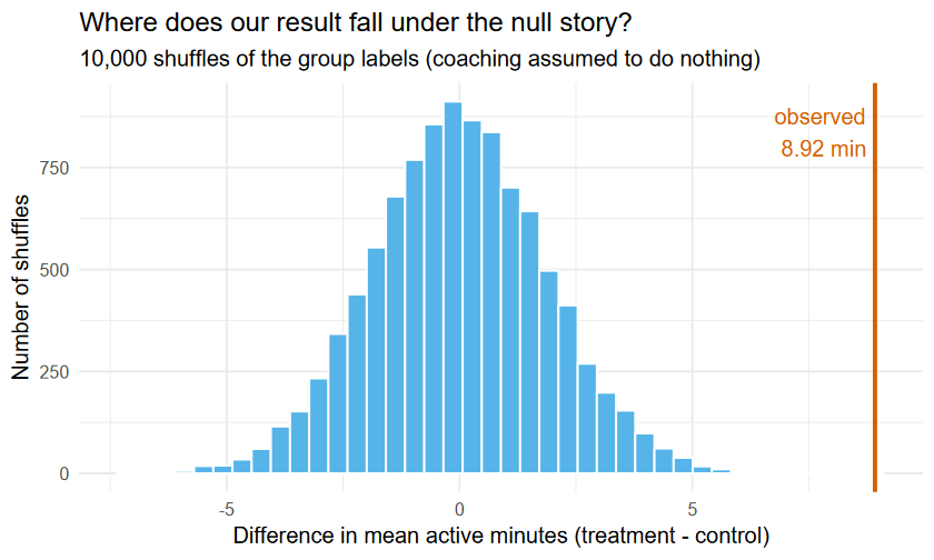
Simulated null distribution of the difference in mean daily active minutes (treatment minus control) from 10,000 random shuffles of the group labels. The histogram is centered at zero with most values between about -5 and +5 minutes. A vertical line marks the observed difference of 8.92 minutes, which lies far to the right of the entire simulated distribution -- no shuffle produced a difference that large -- visually showing why the p-value is below 0.0001.
The observed difference is off the right edge of everything chance produced. The skeptic’s “maybe it’s just luck” story cannot account for a gap this big. We reject .
53. The p-value: what it is, and what it is not
5.1Intuition
The p-value is the single most misread number in statistics, so we will be very careful. It answers one specific question:
If the null hypothesis were true, what is the probability of getting a result at least as extreme as the one we actually observed?
Small p-value our data would be surprising in a world where is true evidence against . Large p-value our data are unremarkable under no evidence against it.
The direction of the conditional is everything. The p-value is the probability of the data, computed assuming the null. It is not the probability that the null is true.
5.2Formula (notation)
The vertical bar “” reads “given.” Read left to right: the probability of an extreme statistic, given . Reversing it — “the probability is true given the data” — is a different quantity entirely, and the test does not compute it.
5.3In R
Our randomization p-value was . We can summarize the evidence compactly:
cat("Observed difference D_obs :", round(obs_diff, 3), "minutes\n")
cat("Shuffles M                :", M, "\n")
cat("Shuffles >= |D_obs|       :", sum(abs(null_diffs) >= abs(obs_diff)), "\n")
cat("Two-sided p-value :", format(p_value), " (report as < 1e-04)\n")64. Decisions, , and the two ways to be wrong
6.1Intuition
A test ends in a decision: reject or fail to reject . In plain words, “reject ” means the data are surprising enough that we stop believing the boring “nothing is going on” story; “fail to reject ” means the data are not surprising enough to abandon that story — so we keep it, for now. (Never “accept ” — we only ever fail to find enough evidence against it; that is a real difference, not word-play, and Q1 of the FAQ explains why.) To decide, we pick a threshold in advance called the significance level, written (“alpha”). is just how surprising the data must be before we are willing to reject . The usual choice is . The rule is simple:
Because we are deciding under uncertainty, we can be wrong in two ways. Picture a smoke alarm:
A Type I error is a false alarm: the alarm shrieks but there is no fire. In testing, that is rejecting when is actually true — declaring an effect that isn’t real.
A Type II error is a missed fire: the house is burning and the alarm stays silent. That is failing to reject when is actually true — missing a real effect.
6.2Formula (notation)
— the significance level, and the long-run probability of a Type I error. By choosing you accept a 5% false-alarm rate when the null is true.
(“beta”) — the probability of a Type II error.
Power — the probability of correctly detecting a real effect. Bigger samples and bigger true effects raise power.
The two errors trade off. Lowering (say to 0.01) makes false alarms rarer but missed fires more common (larger ). You cannot drive both to zero at once; you choose the balance that fits the stakes.
| is true | is false | |
|---|---|---|
| Reject | Type I error () | Correct (power ) |
| Fail to reject | Correct | Type II error () |
6.3In R
Here is made tangible. We simulate a world where is exactly true — random labels on numbers that share one common distribution — and check how often a 5%-level test cries “effect!” anyway. It should be about 5%.
set.seed(2200)
# A population where the null is TRUE: everyone is drawn from the SAME distribution.
type1_flags <- replicate(2000, {
  y  <- rnorm(200, mean = 30, sd = 12)             # no real group difference
  g  <- sample(rep(c("trt", "ctrl"), each = 100))  # random labels
  p  <- t.test(y ~ g)$p.value                       # quick theory-based test
  p < 0.05                                          # did we (wrongly) reject?
})
mean(type1_flags)   # empirical Type I error rate ~ 0.05
The false-alarm rate comes out near 0.05, exactly as promises: when the null is true, a 5%-level test still rejects about one time in twenty. That is the price of the method, fixed in advance — and the reason a single “significant” result is never the end of the story.
75. Significance vs. importance, and the conditions
7.1Intuition
A result can be statistically significant (small p-value: unlikely to be chance) yet practically trivial (the effect is too small to matter). The two are different questions, and you need both:
Statistical significance asks: is the effect real, or just noise? (the p-value).
Practical significance asks: is the effect big enough to care about? (the effect size and its confidence interval).
The villain that lets them diverge is sample size. With a large enough , any nonzero difference — however tiny — eventually becomes statistically significant, because the standard error shrinks toward zero. So “significant” on a huge dataset can mean “real but minuscule,” and “not significant” on a tiny dataset can mean “we couldn’t tell.” Always report the effect size alongside the p-value.
Tests also rest on conditions. For the randomization test the key one is that the grouping was, in the null world, exchangeable — most cleanly guaranteed by random assignment (which our experiment has). For the theory-based two-sample test (Section 6) the conditions are independence (within and between groups) and approximate normality of each group’s distribution (automatically satisfied for the means when each , by the CLT of Chapter 6). Violating independence is the most damaging: it invalidates the standard error, and a test with the wrong standard error gives the wrong p-value.
7.2Formula (notation): a simple effect size
One common effect size for a difference of means is Cohen’s , the difference expressed in pooled-standard-deviation units:
— the pooled standard deviation, a weighted blend of the two group SDs () using their sample sizes (). Think of it as a class-size-weighted average of the two spreads: the bigger group’s SD, being estimated from more data, counts for more.
— how many standard deviations apart the group means are. Rough field conventions: small, 0.5 medium, 0.8 large.
7.3In R
x1 <- active[grp == "treatment"]; x2 <- active[grp == "control"]
n1 <- length(x1); n2 <- length(x2)
sp <- sqrt(((n1 - 1) * var(x1) + (n2 - 1) * var(x2)) / (n1 + n2 - 2))
cohens_d <- (mean(x1) - mean(x2)) / sp
round(cohens_d, 3)
Cohen’s — close to a large effect. So our coaching result is both statistically significant () and practically meaningful (a near-large effect of about 8.9 extra active minutes a day). That is the conclusion you want to be able to defend: not just “significant,” but “significant and sizable.”
86. Connecting the test to a confidence interval
8.1Intuition
A hypothesis test and a confidence interval are two views of the same evidence. A 95% confidence interval for the difference in means is the set of difference-values that a two-sided test at would not reject. So there is a clean equivalence:
The 95% CI for the difference excludes 0 the two-sided test rejects at .
If 0 is a plausible value for the difference (inside the interval), you cannot rule out “no effect.” If 0 is not plausible (outside the interval), you reject “no effect” — and the interval additionally tells you how big the effect plausibly is, which the p-value alone never does.
8.2Formula (notation)
The theory-based (Welch) two-sample interval and test use
where is the standard error of the difference, is the critical
value from the -distribution (Chapter 10 develops this fully), and the
piece is the margin of error. We let mosaic’s t.test() do the
arithmetic; its printout puts the test (the statistic and p-value) and the
confidence interval for the difference side by side.
8.3In R
# Theory-based companion to the randomization test: the Welch two-sample t-test,
# via the mosaic formula active_minutes ~ group.
#
# t.test reports the difference as (first factor level) - (second factor level).
# R orders factor levels alphabetically by default, which would put "control"
# first and report control - treatment (a negative difference). To keep every
# number in this chapter in the intuitive *treatment minus control* direction --
# matching the 8.92-minute gap and the randomization test above -- we make
# "treatment" the first level once, here, and reuse it for the sleep example.
fit$group <- factor(fit$group, levels = c("treatment", "control"))

# t.test prints the test (t, df, p-value), the 95% confidence interval for the
# difference, and each group's mean. With "treatment" as the first level, the
# CI reads treatment - control (positive), exactly as the prose describes.
res <- t.test(active_minutes ~ group, data = fit)
res
The Welch Two Sample t-test block reports (df ),
a p-value of about , a 95% confidence interval for the
difference of about minutes, and the two group means
(mean in group treatment , mean in group control
). The interval lies entirely above 0, so the test rejects
: the two views agree, as they must. And notice what the interval adds: not
merely “the effect is real,” but “the extra active minutes plausibly run from
about 5.5 to 12.4 a day.”
cat("Welch t            :", round(res$statistic, 3), "\n")
cat("p-value            :", format(res$p.value), "\n")
cat("95% CI for diff    : (", round(res$conf.int[1], 3), ",",
    round(res$conf.int[2], 3), ")\n")
cat("CI excludes 0?     :", (res$conf.int[1] > 0 | res$conf.int[2] < 0), "\n")
The randomization p-value () and the theory-based p-value () tell the same story for these data — strong evidence against — which is reassuring: when conditions hold, the simulation and the formula agree.
Going deeper (optional) — why the CI/test equivalence is exact, and the one-sided wrinkle
Skip this box if you are still settling the basics; it is enrichment, not a required skill.
The equivalence “95% CI excludes 0 two-sided test rejects at ” is not a coincidence — it is built from the same standard error and critical value. The two-sided test rejects when
The 95% interval is exactly . So “0 falls outside the interval” and “the test statistic exceeds ” are algebraically the same inequality — same , same . That is why they can never disagree for a two-sided test at the matching level.
The one-sided wrinkle. This clean equivalence is for a two-sided test matched with a two-sided (ordinary) interval. A one-sided test at pairs with a one-sided confidence bound, not the usual two-sided interval — so do not check a one-sided test against a two-sided interval and expect them to line up. And note the duality has limits: the theory-based CI matches the theory-based -test exactly, but the randomization p-value and the -interval are different machines that merely agree closely when conditions hold, as they do here. When you need them to correspond perfectly, match like with like.
9Worked examples
Each example follows the same arc: intuition formula computation interpretation. At least one uses the Kern-relevant classroom dataset.
9.1Example 1 — A borderline result: does coaching change sleep?
(Dataset: fitness_tracker_sim, variable sleep_hours.)
Intuition. The same experiment also recorded average nightly sleep. Coaching might improve sleep, but if it does the effect looks small. This is the interesting case where the answer is “barely.” We test against the two-sided for sleep hours.
Formula. Same randomization machinery as Section 2, with for sleep_hours, and the
two-sided p-value .
Computation.
sleep <- fit$sleep_hours
obs_sleep <- mean(sleep[grp == "treatment"]) - mean(sleep[grp == "control"])

set.seed(2200)
null_sleep <- replicate(10000, {
  s <- sample(grp)
  mean(sleep[s == "treatment"]) - mean(sleep[s == "control"])
})
p_sleep <- mean(abs(null_sleep) >= abs(obs_sleep))

cat("Observed difference :", round(obs_sleep, 3), "hours\n")
cat("Randomization p     :", round(p_sleep, 4), "\n")

# Theory-based companion (Welch t) for the matching confidence interval.
# fit$group still has "treatment" as its first level (set in Section 6),
# so this difference and CI also read treatment - control (positive).
res_sleep <- t.test(sleep_hours ~ group, data = fit)
res_sleep
Interpretation. The observed difference is about 0.273 hours (≈ 16 minutes) more sleep in the treatment group. The randomization p-value is about 0.043, and the Welch test gives with a 95% CI of about hours. Both p-values are just under 0.05, and the CI’s lower end (0.003) sits just above 0 — the test rejects , but only barely, and the effect could be as small as a couple of minutes a night. This is the textbook “statistically significant but practically marginal” verdict: a real-but-tiny effect that a careful analyst would flag as not robust and too small to be sure it matters, the opposite of the decisive active-minutes result. A different random seed could nudge the p-value to either side of 0.05 — which is precisely why the 0.05 line is a convention, not a cliff.
9.2Example 2 — A one-sided test on resting heart rate
(Dataset: fitness_tracker_sim, variable resting_hr.)
Intuition. Physiologically, more activity should lower resting heart rate, so here a directional prediction is justified in advance. We test against the one-sided (treatment lower).
Formula. For a one-sided “less” alternative, the p-value counts only shuffles at least as low as the observed difference: .
Computation.
hr <- fit$resting_hr
obs_hr <- mean(hr[grp == "treatment"]) - mean(hr[grp == "control"])

set.seed(2200)
null_hr <- replicate(10000, {
  s <- sample(grp)
  mean(hr[s == "treatment"]) - mean(hr[s == "control"])
})
p_hr_one_sided <- mean(null_hr <= obs_hr)   # one-sided "less"

cat("Observed difference :", round(obs_hr, 3), "bpm\n")
cat("One-sided p (<)     :", round(p_hr_one_sided, 4), "\n")
Interpretation. The treatment group’s resting heart rate is about 3.29 bpm lower, and the one-sided randomization p-value is about 0.0008 — far below 0.05. We reject in favor of “coaching lowers resting heart rate.” Because the direction was predicted before seeing the data (on physiological grounds), the one-sided test is legitimate here. Warning: choosing one-sided after peeking at which direction the data went is a form of cheating that secretly doubles your false-alarm rate. Decide the direction first, or stay two-sided.
9.3Example 3 — Reading a published claim (no new data)
Intuition. A press release says: “In a randomized trial of 40,000 shoppers, a new app layout raised average order value by $0.06 (p = 0.001).” Should the company rebuild its app?
Formula. The reasoning is the significance-vs-importance logic of Section 5. With the standard error is tiny, so even a difference yields a large test statistic and a microscopic p-value.
Computation (a back-of-envelope illustration). Suppose order values have . Then for the difference, , giving — actually not significant at that . The point: the verdict hinges entirely on and , not on whether $0.06 matters to a customer.
Interpretation. “p = 0.001” tells you the six-cent difference is probably real; it tells you nothing about whether six cents is worth a redesign. The right follow-up questions are the effect size ($0.06 — trivial per order, but times 40,000 orders?) and the confidence interval for the lift. A statistically significant result on a giant sample is an invitation to ask “how big, and big enough for what?”, never a finished argument. (This example uses no curated dataset; the dollar figures are an illustrative scenario, not data.)
9.4Example 4 — Steps: confirming with two methods
(Dataset: fitness_tracker_sim, variable steps.)
Intuition. Daily step count is the headline fitness measure. We expect coaching to raise it; test two-sided to stay honest, and confirm that the randomization test and the theory-based test agree.
Formula. Randomization p-value (two-sided) as in Section 2, plus the Welch companion.
Computation.
steps <- fit$steps
obs_steps <- mean(steps[grp == "treatment"]) - mean(steps[grp == "control"])

set.seed(2200)
null_steps <- replicate(10000, {
  s <- sample(grp)
  mean(steps[s == "treatment"]) - mean(steps[s == "control"])
})
p_steps <- mean(abs(null_steps) >= abs(obs_steps))

cat("Observed difference :", round(obs_steps, 1), "steps/day\n")
cat("Randomization p     :", round(p_steps, 4), "\n")

res_steps <- t.test(steps ~ group, data = fit)
res_steps
Interpretation. The treatment group walked about 942 more steps per day. The randomization p-value is about 0.0018 and the Welch test gives — the two methods agree closely, both well below 0.05. We reject : coaching raised step count. With a difference near 942 steps (roughly a 13% lift over the control mean of about 7,171), this is a result that is both statistically significant and practically meaningful — the kind of clean win the active-minutes result also gave us, and a useful contrast with the borderline sleep result of Example 1.
10Try it yourself
The single most important idea of this chapter is that a p-value is just the tail proportion of the null distribution. The interactive figure below lets you see that. The blue histogram is a randomization null distribution built exactly as in Section 2 — thousands of shuffled-label differences, all from a world where the null is true. Drag the slider to set a hypothetical observed test statistic ; the figure shades the two-sided tail beyond and reports the simulated p-value as the share of shuffles in that shaded tail. Slide right and watch both the shaded area and the p-value shrink — and notice where the tail proportion crosses 0.05.
Figure 1:The p-value is the tail of the null distribution (simulated). — Drag the slider to set the observed statistic; the shaded two-sided tail is the simulated p-value.
Reinforce this chapter with the matching interactive tools:
Shiny “Statistics Explorer” — One/Two-Sample Tests module. Load
fitness_tracker_sim, pickactive_minutesas the response andgroupas the grouping variable, and run the two-sample test. Every action shows the exact mosaic/BSDA R code it ran, so the app and this book teach identical syntax. Launch withshiny::runApp("shiny-explorer")from the repo root and open the One/Two-Sample Tests tab.Jupyter Lab 8 —
labs/lab08-hypothesis-testing.ipynb(R kernel). The lab walks you through building a null distribution by hand, computing a p-value, and comparing it to the theory-based test, with starter code and a reflection prompt. On JupyterHub, openlab08-hypothesis-testing.ipynb; thefitness_tracker_simdata loads withread.csv("data/processed/fitness_tracker_sim.csv").
11Chapter summary
A hypothesis test weighs two stories: the null (“nothing is going on,” assumed true while we judge) and the alternative (“there’s a real effect”). Hypotheses are about parameters, set before seeing the result.
A randomization (permutation) test builds the null distribution by repeatedly shuffling the group labels, then asks where the observed statistic falls. The p-value is the fraction of shuffles at least as extreme as our result.
The p-value is — not the probability is true, not an effect size. Small p-value evidence against .
Decide by comparing the p-value to the significance level (often 0.05). A Type I error is a false alarm (rate ); a Type II error is a missed effect (rate ); power .
Statistical significance (“is it real?”) and practical significance (“is it big enough?”) are different questions; sample size drives both. Always report an effect size and confidence interval with the p-value.
A 95% CI excluding 0 is equivalent to a two-sided test rejecting at — and the CI additionally says how big the effect plausibly is.
12FAQ
Q1. Why can’t I ever “accept” or “prove” the null hypothesis? Because failing to find evidence against is not the same as evidence for it. A large p-value can mean “no effect,” but it can equally mean “there is an effect, but my sample was too small to detect it.” Absence of evidence is not evidence of absence, so we say “fail to reject,” never “accept.”
Q2. What’s the difference between a randomization test and the -test? They answer the same question by different routes. The randomization test simulates the null distribution by shuffling labels — it needs almost no assumptions when you have random assignment, and you can literally see it work. The -test uses a mathematical formula for the null distribution that relies on conditions (independence, approximate normality). When conditions hold, they agree closely, as Examples 4 and the main text show.
Q3. Is a law? Can I use a different threshold? 0.05 is a convention, not a law. You choose in advance to match the stakes: a smaller (e.g. 0.01) when a false alarm is costly, a larger one when missing a real effect is worse. What you must not do is pick after seeing the p-value to get the verdict you wanted.
Q4. When is a one-sided test okay? Only when you can justify the direction before looking at the data — from theory, prior research, or the logic of the problem (as with resting heart rate in Example 2). Choosing one-sided after seeing which way the data leaned secretly doubles your false-alarm rate and is not legitimate.
Q5. My p-value came out as 0. Is the effect impossible under the null? No. A simulated p-value of means “smaller than this simulation can resolve,” i.e. . Report it that way. Run more shuffles, or use the theory-based test, for a more precise tiny value.
Q6. The result is “significant” — does that mean it’s important? Not necessarily. Statistical significance says the effect is probably real, not that it is large or useful. Check the effect size (e.g. Cohen’s ) and the confidence interval. With a big sample, even a trivial difference can be significant.
Q7. Why do we compare absolute values for a two-sided p-value? Because a two-sided alternative () treats a difference as “extreme” if it is far from 0 in either direction. Comparing counts shuffles that are extreme on the left or the right. A one-sided test counts only one tail.
Q8. What breaks the test if I ignore the conditions? Independence is the big one. If observations are not independent (e.g. repeated measures treated as separate subjects), the true standard error is wrong, so the p-value is wrong — usually too small, giving false alarms. Random assignment protects the randomization test; random sampling and independence protect the theory-based test.
13Practice problems
Problems are auto-numbered. Odd-numbered problems have short answers in the
answer appendix; full worked solutions for every
problem live in the instructor key. Unless stated otherwise, use
and the fitness_tracker_sim dataset
(fit <- read.csv("data/processed/fitness_tracker_sim.csv")).
A note on reproducibility
Every numeric result in this chapter is computed from
data/processed/fitness_tracker_sim.csv with the chapter seed set.seed(2200).
Re-running the chapter reproduces every figure and p-value exactly. The
randomization p-values are simulation estimates; with shuffles
they are precise to roughly , which is why the borderline sleep_hours
result (p ≈ 0.043–0.048) should be read as “right around 0.05,” not as a
sharp verdict.
14Resumen en español
Resumen del capítulo
En este capítulo aprendiste la lógica central de la prueba de hipótesis (hypothesis test): un método para decidir si la diferencia que observaste en tus datos pudo haber ocurrido simplemente por azar, o si refleja un efecto real.
El punto de partida es plantear dos historias en competencia. La hipótesis nula (null hypothesis), , dice que no está pasando nada — cualquier diferencia entre grupos se debe a la suerte del sorteo. La hipótesis alternativa (alternative hypothesis), , dice que sí existe un efecto real. Las hipótesis se escriben siempre en términos de parámetros (parameters) — números fijos de la población, como la media poblacional (population mean) — nunca sobre estadísticos de la muestra como .
Para poner esta idea a prueba usamos una prueba de aleatorización (randomization test): tomamos las 200 observaciones del experimento de coaching del capítulo, mezclamos las etiquetas de grupo al azar miles de veces, y recalculamos la diferencia de medias en cada mezcla. Esas miles de diferencias forman la distribución nula (null distribution) — la variación que el azar solo puede producir. Luego preguntamos: ¿qué fracción de esas mezclas generó una diferencia tan grande como la que observamos? Esa fracción es el valor p (p-value).
En el ejemplo principal, la diferencia observada en minutos activos diarios fue de aproximadamente 8.92 minutos, y ninguna de las 10,000 mezclas la igualó, así que el valor p fue menor que 0.0001. Cuando el valor p es menor que el nivel de significancia (significance level) — que convencionalmente se fija en 0.05 — rechazamos .
Al decidir, puedes equivocarte de dos formas: un error Tipo I (Type I error) es rechazar cuando en realidad es verdadera (una falsa alarma cuya tasa es exactamente ); un error Tipo II (Type II error) es no rechazar cuando la alternativa es verdadera (perder un efecto real). La potencia (power) de la prueba es , la probabilidad de detectar un efecto que existe.
Un hallazgo estadísticamente significativo no siempre es prácticamente importante. Con muestras muy grandes, hasta diferencias minúsculas producen valores p pequeños. Por eso siempre debes reportar el tamaño del efecto (effect size) — como la de Cohen — junto con el valor p. Finalmente, un intervalo de confianza (confidence interval) del 95% que excluye el cero equivale exactamente a rechazar a , y además te dice qué tan grande es el efecto plausiblemente.
En R, la función t.test(active_minutes ~ group, data = fit) realiza la prueba de
Welch y muestra el estadístico , el valor p y el intervalo de confianza del 95%
para la diferencia, junto con la media de cada grupo.