Chapter 12 — ANOVA: Comparing Many Means
MATH 2200 · Introduction to Statistical Concepts and Methods
1Why a fourth way to compare groups?¶
You already know how to compare two groups. In Chapter 10 you ran a two-sample -test: is the average PM2.5 at one Bakersfield monitor different from the average at another? But Bakersfield does not have two air monitors. It has three in the city limits — California Avenue, Golden / M Street, and the Airport (Planz Road) site — plus more in Oildale, Shafter, and the desert towns. A reasonable air-quality question is not “do these two differ?” but “do any of these monitors differ from the rest?”
Here is the real 2023 picture, computed live from the curated EPA dataset
kern_airquality (data/codebooks/kern_airquality.md):
The three monitors’ 2023 average daily PM2.5 readings are 11.93, 13.69, and
12.47 µg/m³ (dataset-derived from kern_airquality; PM2.5 daily_mean for the
857 Bakersfield monitor-days). They are close but not identical. Is that gap
real — a true difference in the air across the city — or just the random
wobble you would expect from sampling a few hundred noisy days at each site?
The honest worry: if you ran a separate two-sample -test for every pair of monitors, each test carries its own 5% false-alarm risk, and the risk of at least one false alarm balloons as you add groups. ANOVA — the ANalysis Of VAriance — answers the single question “are these group means all equal?” with one test at one error rate. This chapter is about that test.
2Learning objectives¶
By the end of this chapter you will be able to:
State the ANOVA hypotheses for comparing three or more group means and explain the role of between-group versus within-group variation.
Conduct a one-way ANOVA in R with
aov()+anova()and interpret the -statistic and its -value in context.Check the ANOVA conditions (independence, approximate normality, roughly equal variances) and judge whether the test is trustworthy.
Explain why a single ANOVA is preferred to many pairwise -tests (the multiple-comparisons problem).
Decide whether a follow-up pairwise comparison is warranted, and interpret it cautiously.
Prerequisite: Chapter 10 (inference for means: the procedures, degrees of freedom, conditions for means inference).
R skills introduced: one-way ANOVA with aov(y ~ g, data =) + anova();
group-means plots with gf_boxplot(); reading and reporting an / ANOVA
table; notes on pairwise follow-up.
Durable skills: quantitative reasoning (decomposing variation) · critical thinking (the multiple-comparisons trap).
312.1 The big idea: comparing variation, not just means¶
3.1Intuition¶
The name is a little backwards. ANOVA compares means, but it does so by analyzing variance. Here is the trick that makes it work.
Picture three groups of dots scattered on a number line — exam scores for three class sections, say. There are two completely different reasons the dots are spread out:
Between-group spread. The three group averages sit at different places. If the flipped section averages 16 and the online section averages 20, that gap pushes the dots apart. This is the signal — the thing you care about.
Within-group spread. Even inside one section, students differ. That scatter around each group’s own average is the noise — ordinary person-to-person variability.
Now the key insight. If the groups truly have the same population mean, then the only reason their sample averages differ at all is luck — the same luck that makes individuals within a group differ. In that world, between-group spread and within-group spread are two estimates of the same thing, and their ratio should sit near 1.
But if the groups really differ, the between-group spread gets an extra push from the genuine mean differences, while the within-group spread does not. The ratio climbs above 1. ANOVA is exactly that ratio:
A big says “the gaps between group averages are too large to blame on the ordinary scatter inside the groups.” A small (near 1) says “everything I see is consistent with one common mean.”
3.2Formula¶
We compare groups (here is the number of groups, e.g. monitors). Let:
= observation in group (one monitor-day’s PM2.5);
= the number of observations in group ;
= the total sample size across all groups;
= the mean of group (the group average);
= the grand mean, the average of all observations pooled together.
We split the total variation into the two pieces from the intuition.
Between-group sum of squares — how far each group mean sits from the grand mean, weighted by group size:
Within-group sum of squares — how far each observation sits from its own group mean:
These add up to the total variation: .
A sum of squares is not yet a fair comparison, because SSB is built from groups and SSW from observations. We divide each by its degrees of freedom — the number of independent pieces of information it rests on:
Dividing gives the two mean squares (these are the two variance estimates):
And the -statistic is their ratio:
Under the null hypothesis (all population means are equal, where is the true mean of group ), follows an -distribution with degrees of freedom. The alternative is : at least one group mean differs from the others — not that they are all different.
The -value is the upper-tail area: the probability of an at least as large as the one we observed, if were true. ANOVA is always one-sided on the right, because only large values are evidence against “all means equal.”
Finally, a plain effect size — eta-squared — reports the share of total variation explained by the grouping:
It runs from 0 (groups explain nothing) to 1 (groups explain everything).
Going deeper (optional) — what the F-ratio is really comparing
Enrichment; skip it without penalty. The intuition said MSB and MSW are “two estimates of the same thing” under . Here is the precise version. The within-group mean square always estimates the common error variance: , whether or not the means are equal — it only ever sees scatter inside groups, which the group differences cannot touch. The between-group mean square estimates something slightly bigger: . So under that extra term is zero, both expectations equal , and hovers near 1. When the means truly differ, the numerator’s expectation inflates while the denominator’s stays put, and is pushed above 1. That is why is a ratio of variances that nonetheless tests a claim about means — and why MSW is exactly the pooled within-group variance you saw promised back in Chapter 10’s two-sample t-test.
3.3R¶
The mosaic/base-R workflow is two steps that follow the formula grammar you
already know: fit the model with aov(response ~ group, data = D), then
print the classic ANOVA table with anova() — sums of squares, degrees
of freedom, mean squares, the -statistic, and its -value. Here is the
Bakersfield question:
air <- read.csv("data/processed/kern_airquality.csv")
bak <- subset(air, pollutant == "PM2.5" & city == "Bakersfield")

# aov(response ~ group): daily_mean broken down by site_name.
fit <- aov(daily_mean ~ site_name, data = bak)
anova(fit) prints the ANOVA table. The one thing it does not print is the
effect size , so we compute that from the table’s sums of squares:
anova(fit)                       # SS, df, MS, F value, and Pr(>F)

# eta-squared effect size = SSB / SST, read from the ANOVA table:
ss <- anova(fit)[["Sum Sq"]]     # c(between, within)
eta_squared <- ss[1] / sum(ss)
round(eta_squared, 4)
The anova(fit) table reports F value = 4.0653 on 2 and 854 degrees of
freedom with Pr(>F) = 0.01749, and the effect size works out to
(all dataset-derived from kern_airquality). Working at a
significance level of (the false-alarm rate you decide to accept,
from Chapter 8), we reject : there is evidence that average daily PM2.5
differs across the three Bakersfield monitors — even though tells us
the monitor explains under 1% of the day-to-day variation. (Air quality swings
far more from day to day — winter inversions, summer dust — than it does from
corner to corner of the city. Both facts are true at once, and ANOVA reports
both.)
412.2 The multiple-comparisons problem¶
4.1Intuition¶
Why not just run a -test on each pair of monitors? With three monitors there are three pairs (California–Golden, California–Airport, Golden–Airport). The trouble is that every test you run is another roll of the false-alarm dice.
If a single test uses , it has a 5% chance of crying “difference!” when there is none. Run several independent tests and the chance that at least one of them raises a false alarm is
where is the number of tests and is the per-test error rate. Watch it grow:
m <- 1:10
fwer <- 1 - (1 - 0.05)^m
data.frame(tests = m, familywise_error = round(fwer, 3))
With pairwise tests the family-wise error rate is already about 0.143 — nearly triple the 5% you thought you were using. With ten groups (45 pairs) you are almost guaranteed a false positive. ANOVA sidesteps this by asking one question — “are all the means equal?” — at one error rate.
4.2Formula¶
The fix, when you do need pairwise answers, is to shrink each test’s threshold so the whole family of tests still totals 5%. The simplest is the Bonferroni adjustment: with comparisons, test each one at a stricter threshold (read “alpha-star,” the adjusted per-test cutoff),
so for three pairs you would require on each. A slightly more powerful, ANOVA-specific method is Tukey’s Honest Significant Difference (HSD), which adjusts all pairwise comparisons jointly. Either way, the principle is identical: more looks demand a stricter bar.
4.3R¶
You almost never compute family-wise rates by hand; you let the procedure do it. But seeing the arithmetic once builds trust:
alpha     <- 0.05
m         <- choose(3, 2)            # number of pairwise comparisons among 3 groups
alpha_adj <- alpha / m
c(comparisons = m, per_test_threshold = round(alpha_adj, 4))512.3 Worked example 1 — Do Bakersfield monitors differ? (Kern data)¶
Intuition. Three city monitors, hundreds of daily PM2.5 readings each, three averages a couple of µg/m³ apart. Is the spread between the monitor averages big relative to the spread within each monitor’s daily readings?
Formula. We need SSB, SSW, the two mean squares, and on df.
Computation. First, look — always plot before you test:
air <- read.csv("data/processed/kern_airquality.csv")
bak <- subset(air, pollutant == "PM2.5" & city == "Bakersfield")

gf_boxplot(daily_mean ~ site_name, data = bak, fill = okabe_ito[1]) %>%
  gf_labs(title = "Daily PM2.5 by Bakersfield monitor (2023)",
          x = "Monitor",
          y = "Daily mean PM2.5 (µg/m³)") %>%
  gf_theme(theme_minimal(base_size = 13))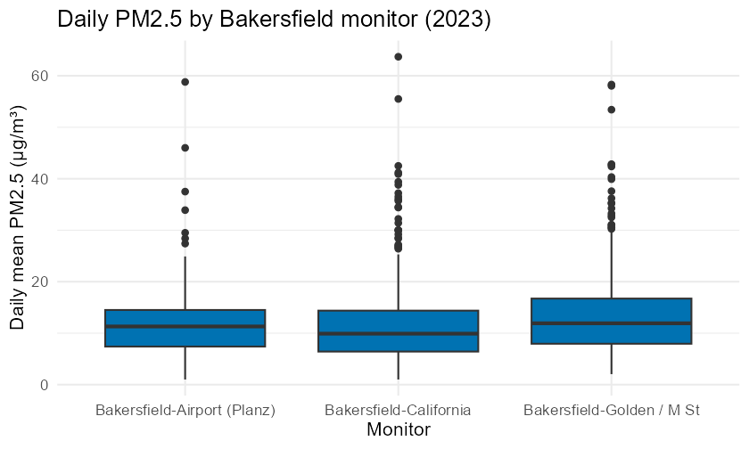
Daily PM2.5 by Bakersfield monitor, 2023. The Golden/M Street box sits slightly higher than the California Avenue box, but all three overlap heavily — a small between-monitor signal inside a large day-to-day spread.
Now the test:
fit1 <- aov(daily_mean ~ site_name, data = bak)
anova(fit1)

# Equal-variance condition: ratio of largest to smallest group SD.
sd_by_site <- favstats(daily_mean ~ site_name, data = bak)$sd
max(sd_by_site) / min(sd_by_site)
Reading the printed ANOVA table (with sums of squares carried to full precision), the computation is:
| Source | SS | df | MS | |
|---|---|---|---|---|
| Between (monitor) | 582.19 | 2 | 291.09 | 4.07 |
| Within (residual) | 61150.74 | 854 | 71.61 | |
| Total | 61732.92 | 856 |
(Sums of squares are dataset-derived from kern_airquality; grand mean
µg/m³.)
Interpretation. , , so we reject : average daily PM2.5 is not the same at all three Bakersfield monitors. To check the equal-variance condition, the second line of the cell above divides the largest group SD by the smallest: the ratio is about 1.04 — comfortably under 2, so the condition is met, and with hundreds of days per group the means are well-behaved. But : the monitor explains under 1% of the variation in daily PM2.5. Statistically detectable, practically tiny — a distinction every honest analyst must report.
612.4 Worked example 2 — Which monitors differ? (pairwise follow-up)¶
Intuition. The ANOVA said “at least one differs.” Fine — which one? We compare pairs, but with a family-wise correction so the three comparisons together still risk only 5%.
Formula. Tukey’s HSD compares each pair’s mean difference against a jointly-adjusted critical distance; equivalently it reports an adjusted -value for each pair that you compare to directly.
Computation. In R the follow-up is TukeyHSD() on the same aov() fit — the
workplace-standard idiom. It reports, for each pair, the difference in means, a
family-wise-adjusted confidence interval, and an adjusted -value (p adj).
air <- read.csv("data/processed/kern_airquality.csv")
bak <- subset(air, pollutant == "PM2.5" & city == "Bakersfield")
bak$site_name <- factor(bak$site_name)   # treat site_name as labeled groups, not text

aov_fit <- aov(daily_mean ~ site_name, data = bak)
TukeyHSD(aov_fit)
Interpretation. Only one pair clears the bar after adjustment:
California Avenue vs. Golden / M Street, with a mean difference of about
1.76 µg/m³ higher at Golden, adjusted (dataset-derived from
kern_airquality). The Airport site is statistically indistinguishable from
either of the other two. So the omnibus “they differ” traces to a single
contrast: Golden/M Street runs dustier than California Avenue. Notice the
discipline — we only earned the right to run these pairwise tests because the
overall ANOVA was significant first.
712.5 Worked example 3 — Crop yields (clear-cut signal, simulated data)¶
The dataset
kern_crops_simis simulated — its name carries the*_simtag so you always know it is made-up (data/codebooks/kern_crops_sim.md). The magnitudes are plausible for Kern agriculture, but they are not measured values. We use it here to show what a large looks like.
Intuition. Compare yield per acre for almonds, pistachios, and oranges. Almonds and pistachios both yield about a ton per acre; oranges, a citrus fruit, yield many tons per acre. The group averages are miles apart compared with the scatter within each crop. Expect a huge .
Formula. Same machinery: on df, with crops and crop-years.
Computation.
crops <- read.csv("data/processed/kern_crops_sim.csv")
three <- subset(crops, commodity %in% c("ALMONDS", "PISTACHIOS", "ORANGES"))
three$commodity <- factor(three$commodity)

fit3 <- aov(yield_per_acre ~ commodity, data = three)
anova(fit3)

# effect size eta-squared = SSB / SST:
ss3 <- anova(fit3)[["Sum Sq"]]
round(c(eta_squared = ss3[1] / sum(ss3)), 4)
Interpretation. with and
(dataset-derived from kern_crops_sim): crop type explains
about 98% of the variation in yield per acre. We reject overwhelmingly —
unsurprising, because the groups barely overlap. Contrast this with the
Bakersfield air example (, ): both are
“statistically significant,” yet one effect is enormous and the other is
hairline. The -value tells you whether there is a difference; the effect
size tells you how much it matters. Always report both.
812.6 Worked example 4 — A pencil-and-paper ANOVA table¶
Intuition. On an exam you will be handed a partial ANOVA table and asked to fill it in and decide. No data, no computer — just the definitions.
Setup. Three training programs, trainees each (). You are told and . Test at .
Formula + computation. With groups:
The completed table:
| Source | SS | df | MS | |
|---|---|---|---|---|
| Between | 48 | 2 | 24 | 4.0 |
| Within | 72 | 12 | 6 | |
| Total | 120 | 14 |
Decision. Compare to the critical value :
qf(0.95, df1 = 2, df2 = 12)      # critical F
pf(4.0, df1 = 2, df2 = 12, lower.tail = FALSE)   # p-value
The critical value is and the -value is 0.0467. Since (equivalently ), we reject : at least one training program’s mean differs. (These two values come from the -distribution, not from a dataset.)
Interpretation. This is the skeleton every ANOVA shares — fill the table, compare to the critical (or compare to ), state a conclusion in context. Practice it until the four boxes (SSB/SSW MSB/MSW decision) are automatic.
912.7 Checking the conditions¶
ANOVA’s -test is trustworthy when three conditions hold. You check all three
yourself — the boxplot and the group standard deviations from favstats() make
the last two quick.
Independence. Observations are independent within and across groups. This comes from the study design, not from the data — a random sample or a randomized experiment earns it. (Daily air readings at one monitor are mildly autocorrelated day-to-day; we treat the monitor-days as approximately independent for teaching, and flag it honestly.)
Approximate normality within each group — or large , in which case the Central Limit Theorem (Chapter 6) covers the group means. With hundreds of days per monitor we are safe.
Roughly equal variances (homogeneity). Compare across the groups (the
favstats()sdcolumn, as in Worked Example 1); a ratio under 2 is the rule of thumb. For the Bakersfield monitors it was about 1.04 — fine.
10Try it¶
Shiny — Statistics Explorer, ANOVA module. Open the ANOVA module of the Statistics Explorer (
shiny-explorer/, module ANOVA). Pickkern_airquality, set the response todaily_meanand the group tosite_name, and watch the live R-code panel print the exactaov()+anova()calls that produced your result — copy them straight into your own script.Jupyter — Lab 12 (ANOVA). Run
labs/lab12-anova.ipynb(R kernel) for a guided walkthrough: build the group-means plot, run the omnibus , then do the Tukey follow-up on a fresh dataset, with starter code and a reflection prompt.Choosing between ANOVA, a two-sample , and the other procedures? The book’s which-test decision guide maps your data (how many groups, what kind of response) to the right test across the whole course.
11Practice problems¶
Work these with mosaic and base R. Odd-numbered problems have short answers
in the appendix (Appendix: Odd Answers); full worked solutions live in the
instructor key. Datasets load with read.csv("data/processed/<name>.csv").
In one or two sentences, state the null and alternative hypotheses for a one-way ANOVA comparing the mean PM2.5 of Kern monitors.
A study compares groups with observations total. Give and .
An ANOVA reports and . Compute and interpret it in one sentence.
True or false, with a reason: “A significant ANOVA means every pair of group means is different.”
Complete the ANOVA table: , , , . Find both , both , and .
For the table in Problem 5, find the critical value with
qf()and state the decision.You run pairwise -tests on all pairs among groups at . How many comparisons is that, and what is the approximate family-wise error rate ?
Explain in your own words why ANOVA uses within-group variation as its yardstick for judging between-group variation.
Load
kern_airquality, keep PM2.5 rows for the three Bakersfield monitors, and reproduce the omnibus ANOVA withaov()+anova(). Report , the two , and .For the Problem 9 fit, report and write one sentence distinguishing statistical significance from practical importance here.
Using
kern_airqualityPM2.5 rows, run a one-way ANOVA ofdaily_meanacross all monitors with at least 100 days (site_name). Report and .Make a boxplot of
daily_meanbysite_namefor the Problem 11 group withgf_boxplot(). In one sentence, does the picture agree with the test?A four-group ANOVA gives and . Compute . If , is it significant at ? (Use
pf().)State the three ANOVA conditions and name the one that comes from study design rather than from the data.
The SD-ratio (max ÷ min group SD) in an ANOVA is 3.1. Which condition is threatened, and what alternative test handles it?
Load
kern_crops_sim, keepALMONDS,PISTACHIOS, andGRAPES, WINE, and runaov()+anova()onyield_per_acre(compute from the table). Report and . (Remember: simulated data.)Why is it invalid to ANOVA almond yield (tons/acre) against cotton yield (bales/acre)? Answer in one sentence.
A significant ANOVA is followed by Tukey HSD; exactly one of three pairs has adjusted . Write the one-sentence conclusion.
Compute the Bonferroni per-test threshold for all pairwise comparisons among groups at family-wise .
Explain why ANOVA’s -test is one-sided (right tail only), referring to what a small near 1 means.
For
kern_airqualityPM2.5, run a Tukey HSD on the three Bakersfield monitors (aov()+TukeyHSD()). Which single pair is significant after adjustment?An ANOVA has and . Compute and comment on whether grouping explains much.
Two analysts test the same 5-group data. One runs ANOVA; the other runs all 10 pairwise -tests at and reports the one “significant” pair. Whose error rate is controlled, and why?
Given , , and an observed , find the -value with
pf()and state the decision at .In one paragraph for a non-technical city official, summarize the Bakersfield PM2.5 ANOVA finding (§12.3–12.4): what differs, by how much, and how much it matters.
12Chapter summary¶
ANOVA compares three or more group means with a single test, avoiding the multiple-comparisons inflation of running many pairwise -tests.
It works by splitting total variation into between-group (SSB) and within-group (SSW) pieces, converting each to a mean square by dividing by its degrees of freedom ( and ), and forming .
Under , follows an -distribution with df. A large (small upper-tail ) is evidence that at least one mean differs — never that all differ.
Report an effect size () alongside the -value: significance and importance are different questions. The Bakersfield monitors differ significantly () yet is under 1%.
Only after a significant omnibus test do you run a family-wise-corrected pairwise follow-up (Bonferroni or Tukey HSD) to find which groups differ.
Check independence (design), approximate normality / large , and roughly equal variances (SD ratio ; otherwise use Welch ANOVA).
13FAQ¶
Q1. Why not just run a -test on every pair? Each test carries its own false-alarm risk, and the chance of at least one false alarm grows as . ANOVA asks one question at one error rate.
Q2. What does a big actually mean? The gaps between group averages are large compared with the ordinary scatter inside the groups — too large to credibly blame on chance.
Q3. ANOVA was significant. Which groups differ? The omnibus test does not say. Run a family-wise-corrected pairwise procedure (Tukey HSD or Bonferroni) after a significant result to locate the difference.
Q4. Is a tiny -value the same as a big effect? No. The Bakersfield air example is significant () but — a real-but-tiny effect. Always report the effect size with the -value.
Q5. My groups have very different spreads. Is ANOVA still valid?
If the SD ratio (max ÷ min) exceeds about 2, the equal-variance condition is
shaky; switch to a Welch ANOVA (oneway.test(..., var.equal = FALSE)).
Q6. Why are there two degrees of freedom? The -distribution is a ratio of two variance estimates, each with its own df: for the numerator (between) and for the denominator (within). Both are needed to find the critical value or -value.
Q7. Can ANOVA compare just two groups? Yes — and it gives exactly the (equal-variance) two-sample -test result, with . ANOVA earns its keep when there are three or more groups.
Q8. Does a significant ANOVA prove the grouping caused the difference? No. Causation requires a randomized experiment. With observational data (like the air monitors) ANOVA establishes a difference, not its cause.
14Resumen en español¶
Resumen del capítulo
En este capítulo aprendiste a comparar las medias (means) de tres o más grupos con una sola prueba estadística llamada ANOVA (Análisis de Varianza, Analysis of Variance). Usar muchas pruebas t separadas inflaría artificialmente la tasa de error: con tres pares, la tasa de error familiar (family-wise error rate) sube a alrededor del 14 % aunque cada prueba use solo el 5 %. ANOVA resuelve esto haciendo una sola pregunta con una sola tasa de error.
La idea central es dividir la variación total de los datos en dos partes. La variación entre grupos (between-group variation, SSB) mide qué tan lejos están los promedios de cada grupo respecto a la gran media (grand mean). La variación dentro de los grupos (within-group variation, SSW) mide el ruido normal que existe dentro de cada grupo. El estadístico es la razón entre ambas: , donde MSB y MSW son las cuadrados medios (mean squares) obtenidos al dividir cada suma de cuadrados entre sus grados de libertad (degrees of freedom).
Bajo la hipótesis nula (null hypothesis) — es decir, que todas las medias poblacionales son iguales — el estadístico sigue una distribución con grados de libertad. Un valor grande produce un valor (p-value) pequeño y nos lleva a rechazar , concluyendo que al menos una media difiere de las demás.
El ejemplo central del capítulo usa datos reales del conjunto kern_airquality: los niveles diarios de PM2.5 en tres monitores de Bakersfield durante 2023. Las funciones aov() y anova() producen , — suficiente para rechazar con . Sin embargo, el tamaño del efecto (effect size) muestra que el monitor explica menos del 1 % de la variación diaria. Un resultado puede ser estadísticamente significativo y aun así ser pequeño en la práctica; siempre debes reportar ambos.
Si el ANOVA global es significativo, puedes identificar cuál par de grupos difiere mediante una comparación múltiple corregida como la Diferencia Honestamente Significativa de Tukey (Tukey’s HSD). Solo el par California Avenue y Golden/M Street resultó significativo: Golden/M Street tiene en promedio 1.76 µg/m³ más de PM2.5 que California Avenue.
Antes de confiar en el , verifica tres condiciones: independencia (independence) de las observaciones, normalidad aproximada (approximate normality) o tamaño de muestra grande, y varianzas aproximadamente iguales (equal variances) — una razón entre la SD máxima y la mínima menor de 2.