1Objectives
By the end of this lesson you will be able to:
Compute and visualize normal probabilities with
xpnorm(), and percentiles withxqnorm(), reading the shaded-curve output each produces.Compute exact and cumulative binomial probabilities with
dbinom()andpbinom(), and visualize a cumulative binomial probability withxpbinom().Compute Poisson probabilities with
dpois()for count data, and compare a theoretical Poisson model to real observed proportions.Simulate probability directly with
do(n) * rflip(...)andsample(), and compare the simulated results to the theoretical probabilities above.Read back, in one sentence, what each probability output means in the context of the question that was asked.
2From “what does the data look like” to “how likely is this”
L07 was about describing data you already have — summaries,
tables, pictures. This lesson turns the question around: if the world
behaves a certain way, how likely is a particular outcome? That “if the
world behaves a certain way” part is a probability model — the normal,
binomial, and Poisson models below are the three this course uses most.
Every model in this lesson is fit either to the running survey_sim dataset
or to the exact parameters its own generator script used, so every
probability you compute here is checkable, not hypothetical. Reload the
toolkit and the data if you’re starting fresh:
suppressMessages({library(mosaic); library(BSDA)})
survey <- read.csv("data/survey_sim.csv")3The normal model: xpnorm() and xqnorm()
The normal model, written , describes a bell-shaped
distribution with mean (its center) and standard deviation
(its spread). L07’s favstats() already gave you a real
and estimate — the sample mean and SD of sleep_hours:
mean(~ sleep_hours, data = survey)
sd(~ sleep_hours, data = survey)
[1] 6.7875
[1] 1.012241xpnorm(q, mean=, sd=) answers “if sleep hours really follow
, what fraction of students sleep more than q
hours?” — and draws the shaded curve, not just the number:
xpnorm(8, mean = 6.7875, sd = 1.012241)
If X ~ N(6.787, 1.012), then

	P(X <= 8) = P(Z <= 1.198) = 0.8845
	P(X >  8) = P(Z >  1.198) = 0.1155

[1] 0.8845098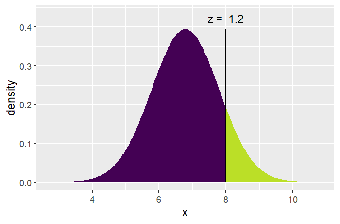
Figure 1:xpnorm() shades P(X <= 8) in purple and P(X > 8) in yellow-green, and labels the standardized cutoff (z = 1.2) on the plot.
Read it the way the console text reads: about 88.45% of students in this
model sleep 8 hours or fewer, so about 11.55% sleep more than 8 hours —
that right-hand sliver is the yellow-green region in the figure. xpnorm()
also returns the lower-tail probability (0.8845098) as an ordinary
number, so you can save it (p_le8 <- xpnorm(8, mean = ..., sd = ...)) and
use it in later arithmetic, same as any other R value.
xqnorm(p, mean=, sd=) runs the question the other direction: given a
probability, find the cutoff. What sleep-hours value marks the top 10% of
the model (the 90th percentile)?
xqnorm(0.90, mean = 6.7875, sd = 1.012241)
If X ~ N(6.7875, 1.012241), then

	P(X <= 8.084739) = 0.9
	P(X >  8.084739) = 0.1

[1] 8.084739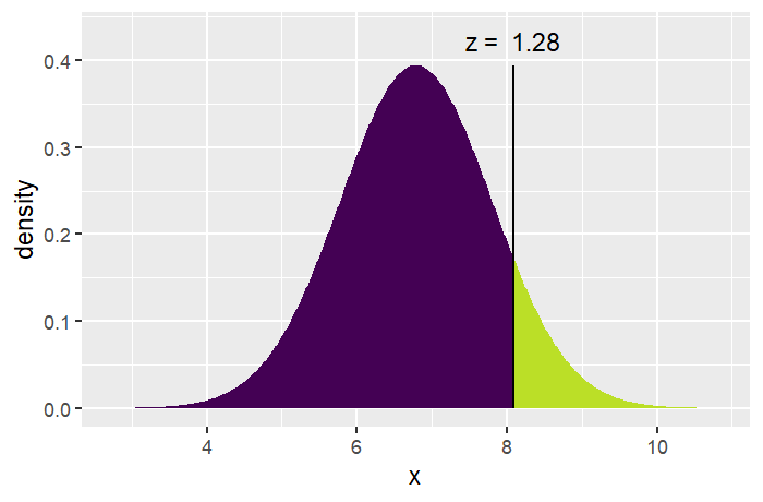
Figure 2:xqnorm() finds the cutoff (about 8.08 hours) that leaves exactly 10% of the model’s area in the upper tail.
About 8.08 hours is this model’s 90th percentile: 90% of students sleep
8.08 hours or fewer, and only 10% sleep more. xpnorm() and xqnorm() are
exact inverses of each other on the same model — feeding xqnorm()'s answer
back into xpnorm() returns you to the probability you started with.
4The binomial model: dbinom(), pbinom(), xpbinom()
The binomial model counts successes in a fixed number of independent
yes/no trials: trials, each with success probability , counting the
number of successes . L07’s pet variable gives us a we
know exactly, because it’s the value the survey’s own generator script
used to create the data (data/make_survey_sim.R): a 46% chance any given
simulated student is a “Dog person.” Imagine sampling 10 students at random
(with replacement) from that population — how many would you expect to be
dog people?
dbinom(x, size = n, prob = p) gives the exact probability of exactly
x successes:
dbinom(5, size = 10, prob = 0.46)[1] 0.2383189About a 23.8% chance that exactly 5 of the 10 are dog people.
pbinom(x, size = n, prob = p) gives the cumulative probability, or
fewer successes:
pbinom(5, size = 10, prob = 0.46)
1 - pbinom(7, size = 10, prob = 0.46)
[1] 0.7167618
[1] 0.03171051About a 71.7% chance of 5 or fewer dog people, and — using the complement
rule, 1 - pbinom(...) — only about a 3.2% chance of more than 7 out of
10. xpbinom() draws the discrete version of xpnorm()'s picture: one dot
per possible outcome, split into two colors at the cutoff.
xpbinom(5, size = 10, prob = 0.46)[1] 0.7167618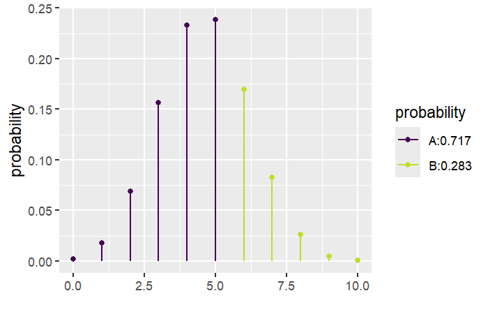
Figure 3:xpbinom() shades P(X <= 5) (purple, “A”) and P(X > 5) (yellow-green, “B”) across every possible outcome of the binomial(10, 0.46) model.
5The Poisson model: dpois()
The Poisson model counts events in a fixed window when the events happen
independently at some average rate (“lambda”) — classic examples
are calls to a help desk per hour, or, in our survey, cups of coffee per
day. coffee_cups in survey_sim was generated from a
model (again, straight from
data/make_survey_sim.R — a real, documented parameter, not a guess).
dpois(x, lambda = ) gives :
round(dpois(0:6, lambda = 1.6), 4)[1] 0.2019 0.3230 0.2584 0.1378 0.0551 0.0176 0.0047According to this model, about 20.2% of students would drink zero cups,
32.3% exactly one cup, 25.8% exactly two, tapering off quickly after that.
Because we generated coffee_cups from exactly this model, the observed
proportions in survey should land in the same neighborhood — a real check
you can run yourself with tally() from L07:
tally(~ coffee_cups, data = survey, format = "proportion")coffee_cups
0 1 2 3 4 5
0.1583333 0.3666667 0.3500000 0.0500000 0.0500000 0.0250000 Close, not identical — 15.8% observed zero-cup students vs. 20.2% theoretical, 36.7% vs. 32.3% at one cup, and so on. That gap is exactly what you’d expect from a sample of only 120 students; a model doesn’t reproduce its own theoretical percentages exactly every time it’s used to generate data, and neither will a real dataset match its true population model exactly. The overall shape — most students at 0–2 cups, dropping off fast after that — clearly matches.
6Simulating probability directly: do(n) * rflip(...) and sample()
Sometimes it’s faster to just simulate an experiment many times and
count, rather than reach for a formula — and simulation is also how you’ll
build intuition for sampling distributions in L09. rflip(n, prob = ) simulates n flips of a coin that lands “heads” with probability
prob (default 0.5, a fair coin); wrapping it in do(1000) * repeats the
whole thing 1000 times. Set a seed first so your simulation is reproducible:
set.seed(2200)
sims <- do(1000) * rflip(10, prob = 0.46)
head(sims, 4)
n heads tails prop
1 10 8 2 0.8
2 10 5 5 0.5
3 10 6 4 0.6
4 10 6 4 0.6Each of the 1000 rows is one simulated “sample 10 students, count dog
people” experiment — n is the number of flips per rep (10, same every
row), heads is how many landed “heads” (dog-person draws) that rep,
tails is the rest, and prop is heads / n. Tally the heads column and
compare it to the exact dbinom() probabilities from the section above:
tally(~ heads, data = sims, format = "proportion")
round(dbinom(0:10, size = 10, prob = 0.46), 4)
heads
1 2 3 4 5 6 7 8 9
0.022 0.074 0.137 0.245 0.243 0.167 0.075 0.033 0.004
[1] 0.0021 0.0180 0.0688 0.1564 0.2331 0.2383 0.1692 0.0824 0.0263 0.0050
[11] 0.0004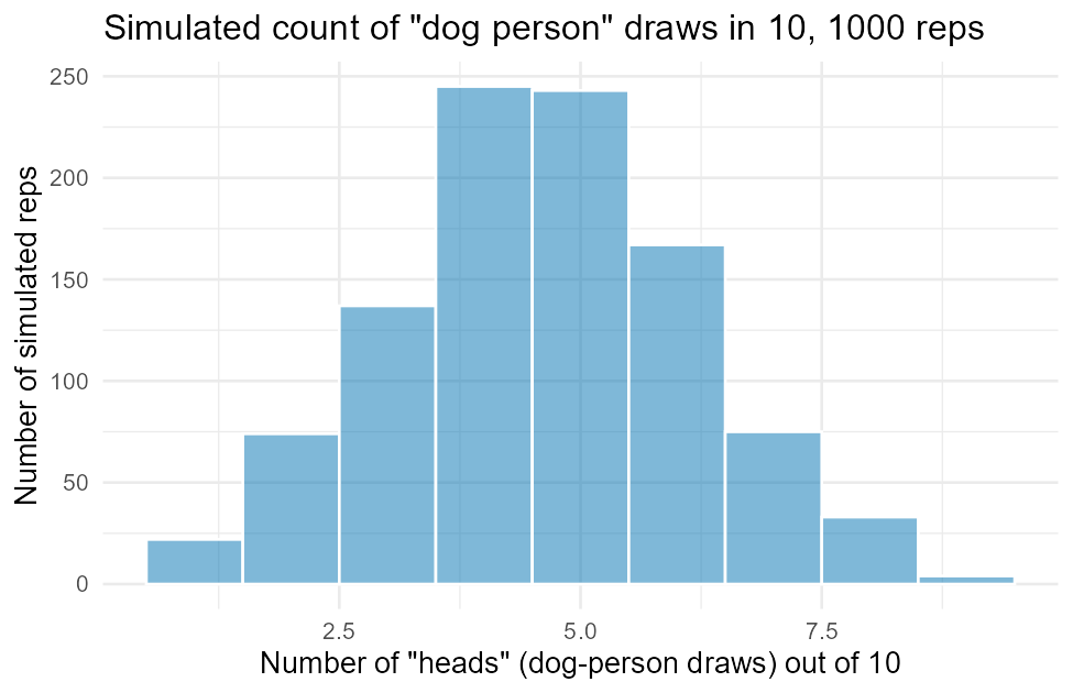
Figure 4:1000 simulated reps of rflip(10, prob = 0.46), closely tracking the theoretical binomial(10, 0.46) shape from the section above.
Read the two tables side by side: the simulated proportion at 5 heads
(0.243) is nearly identical to the theoretical dbinom(5, 10, 0.46)
(0.2383), and the simulated shape peaks in the same place (4–5 heads) as the
theory predicts. Notice heads = 0 and heads = 10 never occurred in these
1000 simulated reps at all — not an error, just sampling luck: dbinom(0, ...) and dbinom(10, ...) are both under half a percent, so in only 1000
tries it’s entirely plausible neither happened. More reps (do(10000) * ...) would fill them in.
sample() is base R’s (also usable inside mosaic) general-purpose random
draw — sample(x, size = , prob = ) draws size values from the vector
x. Simulating a fair six-sided die 1000 times:
set.seed(2200)
rolls <- do(1000) * sample(1:6, size = 1)
tally(~ sample, data = rolls, format = "proportion")
sample
1 2 3 4 5 6
0.140 0.177 0.185 0.195 0.140 0.163 Each face landed close to the theoretical , with the
same kind of simulation noise you just saw for the coin — this is the same
“simulate, then compare to theory” habit, just with sample() standing in
for rflip() when the outcome isn’t a simple heads/tails split.
7Reading probability output: a quick guide
| Function | Question it answers | What it returns/prints |
|---|---|---|
xpnorm(q, mean=, sd=) | P(X ≤ q) and P(X > q) for a normal model | Console sentence + shaded plot + the lower-tail number |
xqnorm(p, mean=, sd=) | What cutoff has probability p at or below it? | Console sentence + shaded plot + the cutoff value |
dbinom(x, size=, prob=) | P(exactly x successes in n trials) | Just the number |
pbinom(x, size=, prob=) | P(x or fewer successes) | Just the number |
xpbinom(x, size=, prob=) | Same as pbinom(), plus a picture | The number + a shaded lollipop plot, no console sentence |
dpois(x, lambda=) | P(exactly x events, rate λ) | Just the number |
do(n) * rflip(k, prob=) | Simulate n reps of k biased-coin flips | A data frame: n, heads, tails, prop per rep |
do(n) * sample(x, size=) | Simulate n random draws from x | A data frame with one column, sample |
8Summary
xpnorm(q, mean=, sd=)andxqnorm(p, mean=, sd=)are inverses on the same normal model: one takes a value and returns a probability (with a shaded curve and a printed sentence), the other takes a probability and returns a value.pnorm()/qnorm()are their plain-number, no-plot equivalents.dbinom(x, size=, prob=)gives an exact binomial probability;pbinom(x, size=, prob=)gives the cumulative version;xpbinom()adds the picture but — unlikexpnorm()— prints no explanatory sentence.dpois(x, lambda=)gives a Poisson probability for count data; comparing a theoretical model’sdpois()values to a real sample’stally(..., format = "proportion")is a genuine, checkable model-fit habit.do(n) * rflip(k, prob=)anddo(n) * sample(x, size=)simulate probability directly — repeat an experiment many times,tally()the results, and compare the simulated proportions to the theoretical values above. The two should agree closely, with the gap shrinking asngrows.The full script that generated every figure and number in this lesson is committed at
data/make_L08_figures.R— run it yourself to reproduce every output exactly.