The Toluca Company builds refrigeration equipment and the replacement parts that keep it running. One part had long been produced in batches, or lots, of whatever size seemed convenient at the time. When the company started a cost-cutting review, its engineers wanted to settle a basic question: what lot size is cheapest to produce? Every production run carries a fixed setup cost that does not care about lot size, plus machining and assembly work that grows with the number of parts. To find the sweet spot, the engineers first needed one ingredient: how do the labor hours a run consumes depend on the size of the lot?
They pulled records from 25 recent runs made under stable conditions over a six-month period. Each record is a pair: the lot size (units produced) and the work hours the run took. The lot sizes are all multiples of ten, a scheduling convenience, and they range from 20 to 120 units. The scatter of these 25 points is the starting picture of the whole chapter.
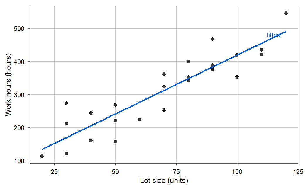
Figure 1:The 25 Toluca runs with the least-squares line drawn through them. Bigger lots take more hours, the trend looks straight, and the scatter around the line is roughly the same width all across, which is exactly the situation this chapter models.
Two things stand out in Figure 1. Bigger lots take more hours, and the cloud of points is close enough to a straight line that a line is a reasonable summary. But which line? An engineer could lay a ruler on the plot and draw one by eye, and a second engineer would draw a slightly different one. This chapter replaces the ruler with a rule: a precise, defensible recipe for the single best line, an honest account of how much to trust it, and the assumptions that make the whole enterprise valid. By the end you will be able to fit that line, read its slope in the units of the problem (hours per unit of lot size), say how uncertain the slope is, and prove that under stated conditions no competing method does better.
The modeling workflow
Every chapter of this book is one pass through the same five-stage loop. Naming the stages now gives you a map to carry through the whole course, and every later chapter opens by saying which stage it serves.
ASK. Fix the question and the data that can answer it. Here: how do work hours depend on lot size, and what can 25 production runs tell us?
EXPLORE. Plot and summarize before fitting anything. The scatter in Figure 1 is this stage; it is what tells us a straight line is even worth trying.
FIT. Estimate the model. Most of this chapter lives here, turning the ruler-and-eye line into the single least-squares line.
CHECK. Ask whether the fitted model can be trusted, using the residuals and the assumptions behind them. We begin this in Section 2.3 and devote all of Chapter 9 to it.
USE. Interpret the estimates, predict, and decide. Reading the slope in hours per unit of lot size is the first taste; inference and prediction fill Chapter 3.

Figure 2:The five stages as one loop. You move clockwise from ASK to USE, and a failed CHECK does not end the work: the dashed arrow sends you back to FIT or EXPLORE with a better model.
As Figure 2 shows, the stages form a loop, not a one-way street: a failed CHECK sends you back to EXPLORE or FIT with a better model. Simple linear regression is the smallest complete trip around this loop, which is why the course starts here.
2.1 The simple linear regression model
Intuition
Regression starts from a plain idea: one thing tends to move with another, and we want to pin that relationship down in numbers. Here we describe how a response (Toluca work hours) depends on a single predictor (lot size). No sane model claims the hours are an exact function of lot size: two runs of the same size took different amounts of time, because of tool wear, the crew on shift, the weather, and a hundred small things nobody recorded. So we split each observation into two pieces: a systematic part that lot size explains, and a random part that it does not.
The systematic part is a straight line. On average, a run of size takes some baseline amount of time plus a fixed number of extra hours per additional unit. The random part is a disturbance that pushes the actual hours above or below that average. We assume the disturbance has no built-in tendency to be positive or negative, has the same typical size regardless of lot size, and does not coordinate from one run to the next.
Formula
The simple linear regression model (Definition 2.1) for observations is
is the observed response in the -th case (work hours for run ).
is the predictor in the -th case (lot size for run ), treated as a known, fixed constant. Some books call this the independent variable or the explanatory variable; this book says predictor throughout.
is the intercept parameter: the mean response when .
is the slope parameter: the change in the mean response for a one-unit increase in .
is the random error in the -th case, the amount by which departs from its mean.
The parameters and are fixed numbers we do not know and want to estimate. The model puts four conditions on the errors:
In words: each error averages to zero (the line is right on average), every error has the same variance (constant spread, called homoscedasticity), and distinct errors are uncorrelated (one run’s luck says nothing about another’s). Notice what is not yet assumed: no particular shape for the error distribution. Normality enters only in 2.6 Maximum likelihood under normal errors, and only when we want to build intervals and tests.
Because is a fixed constant and is therefore also constant, the error conditions transfer directly to the responses:
The quantity is the mean response at level . The function that gives the mean response at any is the regression function (Definition 2.2). It is a line, and estimating it is the whole game.
Figure 3 is the mental picture to carry through the chapter: a straight mean line, with a distribution of possible values stacked at each , every stack the same width.
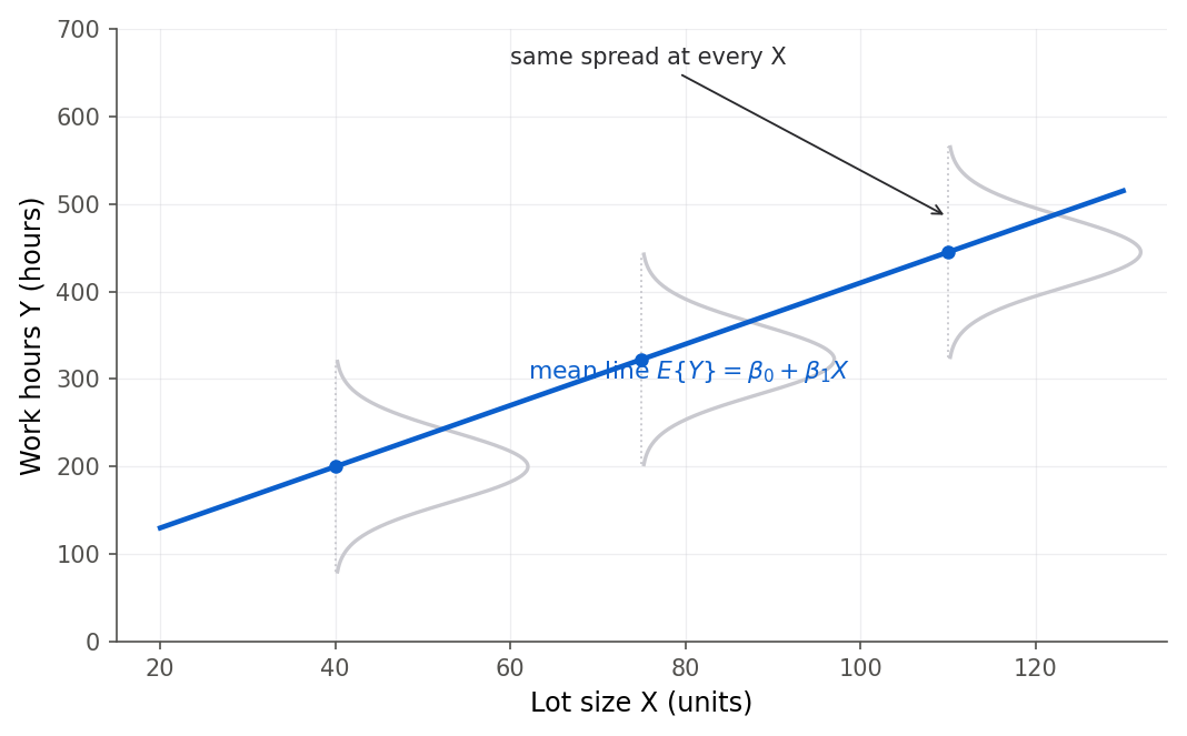
Figure 3:The model in one picture: the mean of Y sits exactly on the line, and at every X the response scatters around that mean by the same amount. The bells are drawn identical on purpose, that is the constant-variance assumption.
2.2 Least squares from first principles
Intuition
We have a cloud of points and want the one line that fits best. “Best” needs a definition. Least squares defines it by penalizing misses: for a candidate line, measure the vertical gap from each point to the line, square the gaps so that overshooting and undershooting both count as errors and large misses hurt disproportionately, and add them up. The best line is the one that makes this total, the sum of squared errors, as small as possible. Figure 4 shows the idea with three candidate lines through the Toluca data.
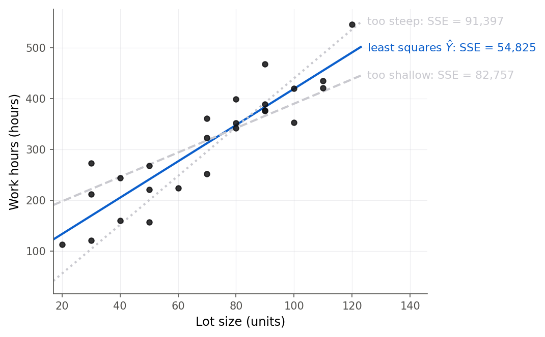
Figure 4:Three candidate lines and their sums of squared errors. The too-shallow and too-steep lines leave large vertical gaps and large SSE; the least-squares line threads the cloud and has the smallest SSE of any line.
Formula
Write a candidate line with intercept and slope . Its sum of squared errors (Definition 2.3) is
is the vertical gap from the point to the candidate line.
is a function of the two numbers we get to choose; the data are fixed.
The least-squares estimates and are the values that minimize . To write them compactly, define the three basic sums of squares and cross-products around the means:
where and are the sample means of the predictor and response. The next two derivations establish the minimizers, stated here first.
Derivation by calculus
Proof (by calculus). is a sum of squares, so it is smooth and bounded below by zero. At a minimum, both partial derivatives vanish. Differentiate:
Setting each to zero and dividing by -2 gives the normal equations:
Expand the sums. The first equation becomes , and dividing by gives , so
Substitute this into the second normal equation . Replacing and collecting the terms,
The left side equals , and the right side’s bracket equals . Therefore
This is the only stationary point, and it is a minimum by the second-derivatives test for a function of two variables (the same test you would use in calculus for one variable, extended to two). The three second partial derivatives of are constants: , , and . Form the test quantity . Since whenever the are not all equal, and , the stationary point is a local minimum. Because is a sum of squares (so it is bounded below by zero) and this is its only stationary point, that local minimum is also the global minimum. (Chapter 7 revisits this same fact in matrix form, once you have the tools of Chapter 6.)
Derivation by an algebraic identity
The calculus argument finds the minimizer but leaves the geometry a little hidden. Here is a second proof that uses no derivatives and shows directly that no line beats the least-squares line. It rests on two facts we will prove in 2.3 Fitted values and the properties of residuals: writing the fitted values as and the residuals as , the residuals satisfy and .
Proof (by an algebraic identity). Take any competing line with intercept and slope . Split the gap from each point to that line by routing it through the least-squares fitted value:
Square and sum. The sum of squared errors for the competing line is
The cross term vanishes:
So for every competing line,
with equality only when , that is when for all , which (since the are not all equal) forces and . The least-squares line is the unique minimizer.
The two normal equations have a clean picture. Each one is a line in the plane, and the least-squares estimates sit where they cross, at the bottom of the SSE bowl. Figure 5 shows the bowl and Figure 6 shows it from above.
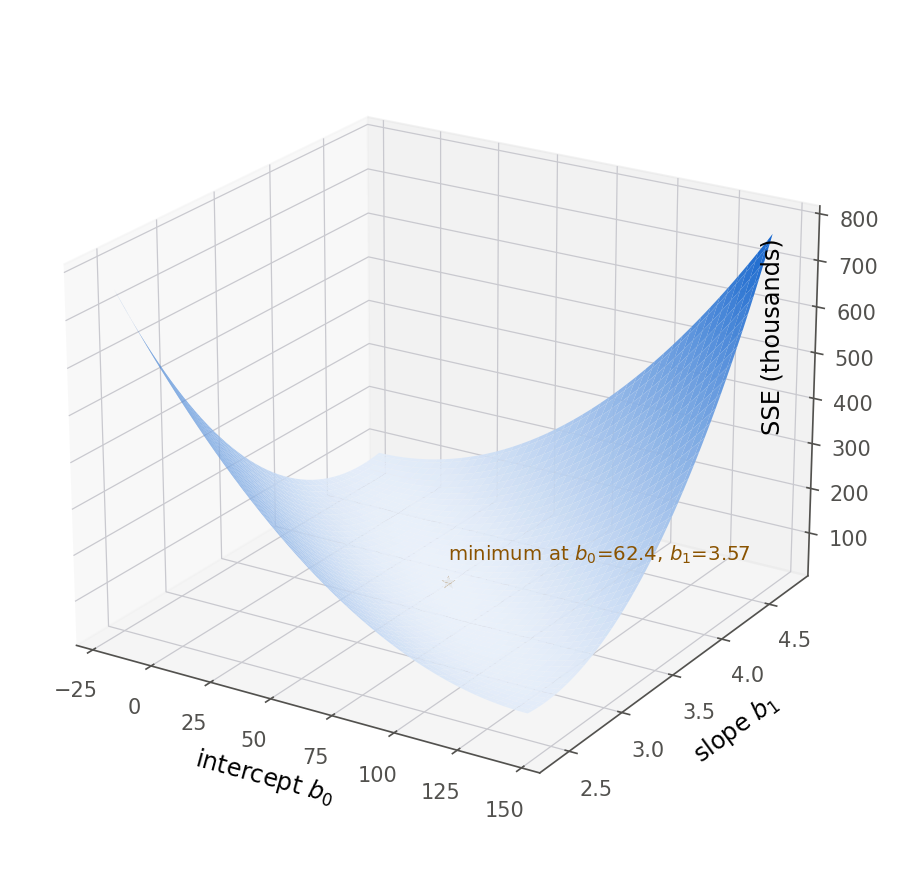
Figure 5:Because SSE is a convex (bowl-shaped) function of the intercept and slope, it has exactly one lowest point, and that point is the least-squares solution. There are no other valleys to get stuck in.
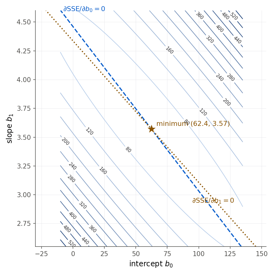
Figure 6:The same SSE surface seen from directly above. Each normal equation is a straight line in the (b0, b1) plane; the two lines intersect at the star, the least-squares estimates, sitting at the center of the innermost contour.
R
Fitting the model in R uses lm, which reads a formula response ~ predictor. First read the
data and look at it.
toluca <- read.csv("data/toluca.csv")
dim(toluca)
head(toluca, 3)
[1] 25 2
lotsize hours
1 80 399
2 30 121
3 50 221Being able to reproduce lm from the raw sums and matters: it means you can
compute a regression anywhere, check software output, and, later, extend the idea when there is
no lm button for the model you need.
Small datasets are worth computing by hand once, so the formulas stop being black boxes. The
file toluca_mini.csv is a six-row slice of the Toluca data, small enough to do on paper.
Figure 7 shows its points and their deviations from the means, the raw material
of and .
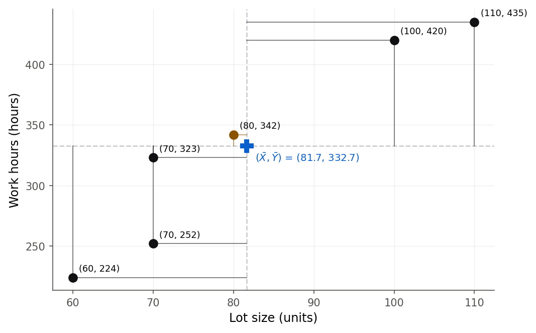
Figure 7:The six hand-computation points with the mean cross drawn in. A point’s horizontal deviation times its vertical deviation is its contribution to Sxy; most points sit in the two quadrants where that product is positive, so Sxy and the slope come out positive.
Before you take the formulas on trust, spend a minute trying to beat them by hand.
Two sliders set your own intercept and slope on the 25 Toluca runs. The readouts compare the your line achieves against the smallest value any line can achieve.
What to notice. No pair of slider settings pushes below , and the settings that come closest read 62.5 and 3.57, the least-squares estimates. Try this. Hold the slope at 3.57 and sweep the intercept alone: the sum of residuals crosses zero at exactly the setting where bottoms out, which is the first normal equation happening in front of you. Back to Section 2.2.
2.3 Fitted values and the properties of residuals
Intuition
Once the line is fixed, every observed point splits into two parts. The fitted value (Definition 2.5) is where the line says the point should be; the residual is how far the actual point lands from it. Residuals are the model’s leftovers, the part of that lot size did not explain. Figure 9 draws them as the vertical sticks connecting each point to the line. They are not just scenery: least squares forces the residuals to satisfy exact algebraic identities, and those identities are both a proof tool and a practical way to catch a mistake in a fit.
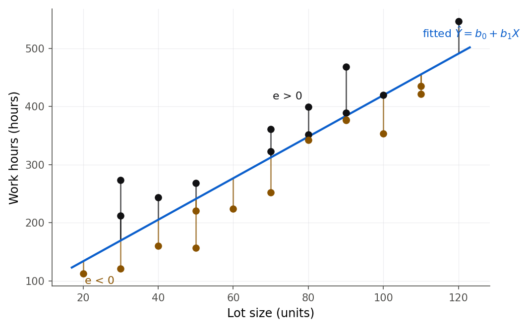
Figure 9:Each residual is the signed vertical distance from a point to the fitted line: positive (orange, above) or negative (purple, below). Least squares balances them so the signed residuals sum to exactly zero.
Formula
The fitted values and residuals are
is the estimated mean response at , the height of the fitted line there.
is the residual, the vertical gap from the observed down to the line.
Do not confuse with the model error . The error is the gap to the true, unknown line; the residual is the gap to our estimated line. We never see , but we can always compute , and it is our best stand-in. Figure 10 puts the two gaps side by side so the difference is impossible to miss.
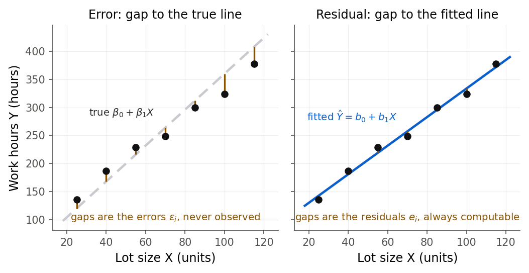
Figure 10:The one distinction to keep straight: the error is the gap to the true line we can never see (left), and the residual is the gap to the fitted line we compute from the data (right). Same points, two different lines, two different gaps.
Derivation (properties of residuals)
Proof. All of these follow from the two normal equations of 2.2 Least squares from first principles.
The residuals sum to zero. The first normal equation is exactly .
The predictor is orthogonal to the residuals. The second normal equation is exactly .
The fitted values are orthogonal to the residuals. Using properties 1 and 2, .
The fitted values reproduce the total of . From property 1, , so , and dividing by , the mean fitted value equals .
The line passes through the center of the data. Setting in the fitted line and using gives . So is always on the least-squares line.
Property 1 is why the vertical sticks in Figure 9 balance out. Properties 1 and 2 were the ingredients that made the cross term vanish in the algebraic proof of 2.2 Least squares from first principles, so the identities repay the loan we took there.
R and Python
A plot of the residuals against the predictor is the first picture to draw after any fit. If the model’s constant-variance and straight-line assumptions hold, the residuals should hover around zero with no trend and no fanning, as in Figure 11. A curve would signal that the relationship is not straight; a widening funnel would signal nonconstant variance. Chapter 9 builds a full diagnostic toolkit on this one habit.
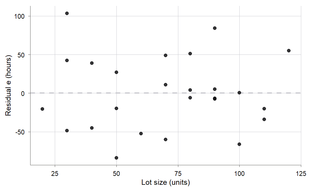
Figure 11:The Toluca residuals plotted against lot size. They sit in a flat, patternless band around zero with no funnel shape, which is the picture that supports the straight-line and constant-variance assumptions.
The identities in Theorem 2.6 are exact, so the fastest way to believe them is to try to break one.
Drag any of the six hand-computation runs anywhere on the plot. The line refits instantly, and the four readouts track , , the mean of , and the mean of .
What to notice. However badly you mangle the data, and stay at zero and the mean of stays equal to . Try this. Drag one run to the very top of the plot: the residuals become huge, the fit becomes useless, and the identities do not move, which is why they check your arithmetic and never your model. Back to Section 2.3.
2.4 Estimating the error variance
Intuition
The slope and intercept describe the line, but the model has a third unknown: , the variance of the errors, which controls how tightly the points hug the line. A small means predictions can be sharp; a large one means even a perfect line leaves big uncertainty. We cannot see the errors , but the residuals are their visible stand-ins, so we estimate from the spread of the residuals. Figure 13 shows what that spread looks like as a band around the fitted line.
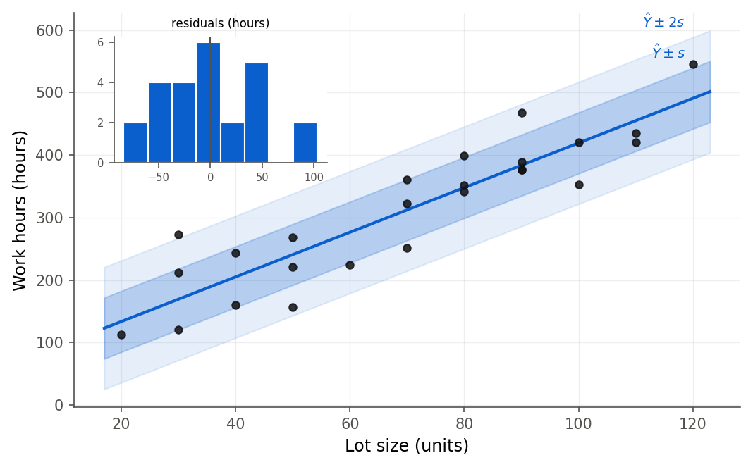
Figure 13:The estimated error spread s = 48.8 hours drawn as bands around the fitted line. About two-thirds of the runs fall within one s of the line and almost all within two s; s summarizes the width of the residual histogram in the inset.
Formula
The error sum of squares (Definition 2.7) and the estimator of are
is the total squared residual, the leftover variation the line did not explain.
(mean square error), also written , is divided by its degrees of freedom ; it estimates .
is the estimated standard deviation of the errors, in the units of (hours).
The divisor is , not or . Two degrees of freedom are spent estimating the two coefficients and that define the line the residuals are measured from. The next derivation shows that this exact divisor, and no other, makes correct on average.
Derivation (why the divisor is )
Proof. We show , so that dividing by gives an estimator that is right on average. Start from a tidy identity for SSE. Since (using ),
so, expanding the square and using ,
Take expectations of the two pieces. For any random variable, .
The slope piece. We show in 2.5 Sampling behavior and the Gauss-Markov theorem that and . Hence
The total piece. Write . Each has mean and variance , so and . The sample mean has mean and variance , so . Subtracting,
The final bracket is . So .
Combine. Subtracting the slope piece from the total piece,
Therefore : the divisor is exactly what makes an unbiased estimator of .
R and Python
Theorem 2.8 says the divisor is the one that is right on average, and repeated sampling is the way to watch that claim settle.
Each sample is 25 fresh runs from a model whose error variance really is . The histogram collects , and the readouts show what each divisor gives on average.
What to notice. Individual values of scatter widely, most of them landing anywhere from about 1200 to about 4000, yet their average walks steadily toward 2383.4. Try this. Press Draw 1000 twice and compare the two means: the divisor lands on while the divisor stays about 8 percent low no matter how many samples you add, which is what bias means. Back to Section 2.4.
2.5 Sampling behavior and the Gauss-Markov theorem
Intuition
The estimates and are computed from a particular sample of 25 runs. A different 25 runs, made under the same conditions, would give slightly different estimates. So and are themselves random: they have distributions, called sampling distributions, across the repeated samples we could have drawn. Figure 15 makes this concrete by simulating 60 fresh samples at the Toluca lot sizes and fitting each: the fitted lines scatter around the true mean line, and they fan out most where is far from .
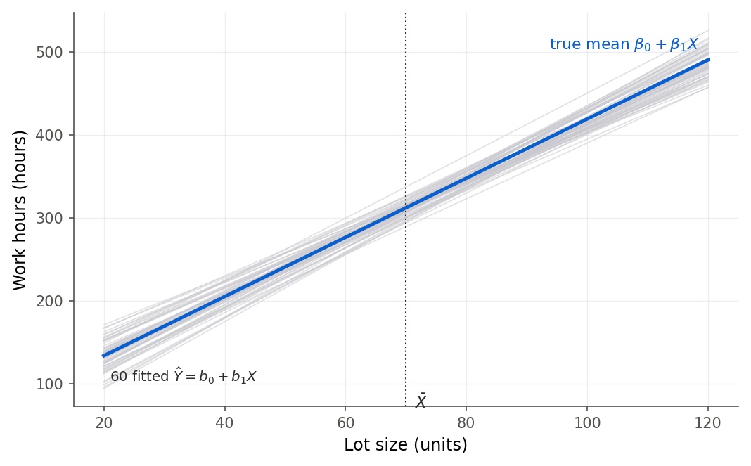
Figure 15:Sixty samples, sixty fitted lines. They cluster around the true mean line (red) with no systematic offset, and the bundle pinches in at the mean lot size and widens at the extremes, which is exactly what the variance formulas predict.
Two questions organize this section. Are and correct on average (unbiased)? And how much do they vary from sample to sample (their variances)? The Gauss-Markov theorem then delivers a strong payoff: among all the sensible estimators one might invent, least squares has the smallest variance.
Formula
Both estimators are unbiased, and their variances are
shrinks when the errors are small ( low) or the predictor is spread wide ( large). Spreading your values out buys precision.
carries an extra term because the intercept lives far off at , and tilting the line pivots it there.
Figure 16 makes the first fact visible. When the lot sizes are bunched together, a little noise tips the slope wildly; when they are spread wide, the same noise barely moves it.
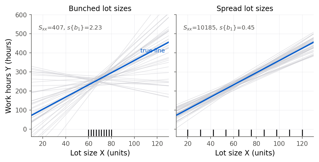
Figure 16:Why spreading X out buys precision. Both panels use the same true line and the same error size; only the spread of the lot sizes differs. Wide spread (right) makes Sxx large, and since the slope variance is sigma squared over Sxx, the slope is pinned down far more tightly.
Replacing the unknown by its estimate gives the estimated variances and , whose square roots are the standard errors and that software prints.
Derivation (unbiasedness and variances)
Proof (mean and variance of ). The key is to write as a weighted sum of the responses. Since ,
The weights depend only on the fixed values and satisfy three facts, each a one-line computation:
Unbiasedness. Using ,
Variance. The are uncorrelated with common variance , so variances of a weighted sum add with squared weights:
Proof (mean and variance of ). Write with . Then and , so . For the variance, using and ,
Derivation (Gauss-Markov: is BLUE)
Proof. Consider any linear estimator with fixed weights . Its expectation is . For this to equal for every possible and , the weights must satisfy
Write , splitting each weight into the least-squares weight and a deviation . Because both and satisfy the two unbiasedness constraints, the deviations satisfy and . Now the cross term drops out:
Therefore
Since , every linear unbiased competitor has variance at least that of , with equality only when all , that is when the competitor is . The least-squares slope is BLUE. The same argument with weights shows is BLUE.
R and Python
The variance formulas are not just algebra; they describe the fanning bundle of lines in Figure 15. We can confirm both the unbiasedness and the slope-variance formula by simulation, drawing 5000 samples from the estimated model and refitting each. Figure 17 shows the histogram of the 5000 slope estimates.
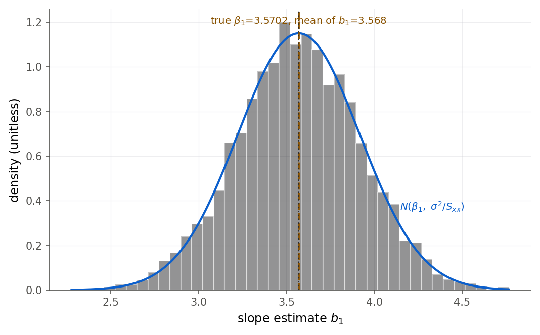
Figure 17:Five thousand simulated slope estimates. Their average lands on the true slope (the dashed and dotted lines nearly coincide), confirming unbiasedness, and their spread matches the theoretical sigma over root Sxx curve, confirming the variance formula.
set.seed(4210)
beta0 <- 62.366; beta1 <- 3.5702; sigma <- 48.82
xfix <- toluca$lotsize
Sxx_fix <- sum((xfix - mean(xfix))^2)
b1_sim <- replicate(5000, {
  ysim <- beta0 + beta1 * xfix + rnorm(length(xfix), 0, sigma)
  coef(lm(ysim ~ xfix))[["xfix"]]
})
round(c(mean_of_b1_hats = mean(b1_sim),
        true_beta1 = beta1,
        sd_of_b1_hats = sd(b1_sim),
        formula_se = sqrt(sigma^2 / Sxx_fix)), 4)
mean_of_b1_hats true_beta1 sd_of_b1_hats formula_se
3.5699 3.5702 0.3479 0.3469rng = np.random.default_rng(4210)
beta0, beta1, sigma = 62.366, 3.5702, 48.82
xfix = toluca["lotsize"].to_numpy()
Sxx_fix = np.sum((xfix - xfix.mean()) ** 2)
b1_hats = np.empty(5000)
for i in range(5000):
ysim = beta0 + beta1 * xfix + rng.normal(0, sigma, size=xfix.size)
b1_hats[i] = np.polyfit(xfix, ysim, 1)[0]
print(round(b1_hats.mean(), 4), beta1,
round(b1_hats.std(ddof=1), 4),
round(np.sqrt(sigma ** 2 / Sxx_fix), 4))3.5675 3.5702 0.352 0.3469The average of the 5000 slope estimates sits right on (unbiasedness), and their simulated standard deviation, 0.348 in R and 0.352 in Python, matches the formula value . The two languages differ only in the last digit because they use different random number generators; the agreement with theory is the point.
The bundle of fitted lines in Figure 15 is easier to believe when you build it one sample at a time.
Every sample reuses the 25 Toluca lot sizes with fresh errors around the line . The strip on top is the newest sample of work hours; the histogram below collects the fitted slope from all of them.
What to notice. Draw samples one at a time and no single equals 3.5702, yet the pile they build is centered there. Try this. Press Draw 1000 and compare the SD of readout with sitting beside it: the variance formula of Theorem 2.9 is not an approximation, it is the width of this pile. Back to Section 2.5.
2.6 Maximum likelihood under normal errors
Intuition
So far we chose least squares because squared error is a reasonable penalty, and Gauss-Markov rewarded that choice with the best-linear-unbiased property, all without assuming any shape for the error distribution. Now suppose we add one assumption: the errors are normally distributed. A different principle, maximum likelihood, asks which parameter values make the data we actually observed most probable. Remarkably, under normal errors that principle points at the very same line. Figure 19 shows the two criteria, sum of squared errors and negative log-likelihood, bottoming out at exactly the same slope.
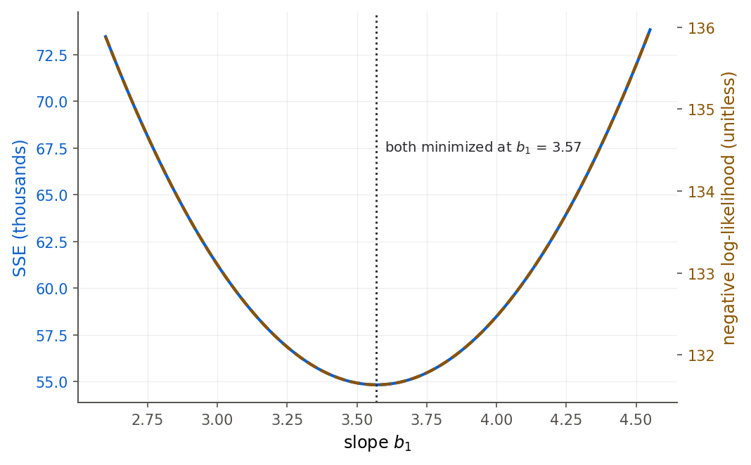
Figure 19:Least squares and maximum likelihood are the same optimization dressed differently. The SSE curve and the negative log-likelihood curve reach their minimum at the identical slope, so choosing the maximum-likelihood line is choosing the least-squares line.
Formula
The normal error regression model (Definition 2.11) keeps everything from 2.1 The simple linear regression model and adds a shape:
Under normality the uncorrelated errors are now fully independent. The likelihood is the joint density of the observed read as a function of the parameters:
is large for parameter values that make the observed data look typical, small for values that make it look freakish.
Maximum likelihood estimates are the that maximize .
Derivation (maximum likelihood equals least squares)
Proof. Maximizing is easier through its logarithm, which is maximized at the same place because is increasing:
Coefficients. Fix any . The first two terms do not involve or , and the last term has multiplying . Maximizing over therefore means minimizing that sum of squares, which is exactly the least-squares criterion from 2.2 Least squares from first principles. So the maximum-likelihood estimates of the coefficients are the least-squares estimates:
Variance. Substitute so the sum of squares becomes , then differentiate with respect to and set it to zero:
The maximum-likelihood variance estimate divides by , not . From 2.4 Estimating the error variance we know the divisor is biased low, understating , because it ignores the two degrees of freedom spent on and . That is why the book, and all the inference in Chapter 3, uses the unbiased rather than the maximum-likelihood .
R and Python
2.7 Chapter summary
This chapter built a simple linear regression from the ground up and proved the properties that make it trustworthy. Starting from the model and its three error assumptions, we defined the least-squares criterion and derived the estimators two independent ways, by calculus through the normal equations and by an algebraic identity that shows no other line has a smaller SSE. The residuals obey exact identities that double as a correctness check; the error variance is estimated by , whose divisor is exactly what makes it unbiased. Treating and as random over repeated samples gave their means and variances, the Gauss-Markov theorem showed they are best among linear unbiased estimators with no normality needed, and maximum likelihood under normal errors reproduced the very same line.
Key results at a glance
| Result | Statement or formula | Valid when |
|---|---|---|
| Least-squares estimates (Theorem 2.4) | , | the are not all equal |
| Residual identities (Theorem 2.6) | , , , | any least-squares fit with an intercept |
| Error variance estimate | , with | SLR model |
| Unbiasedness of MSE (Theorem 2.8) | , so | mean-zero, constant-variance, uncorrelated errors |
| Means and variances (Theorem 2.9) | ; | SLR model |
| Gauss-Markov theorem (Theorem 2.10) | are BLUE (minimum variance among linear unbiased estimators) | SLR model, no normality needed |
| Maximum likelihood (Theorem 2.12) | MLE coefficients ; | normal error model |
For the Toluca data these give , , , , , , , and .
Key terms
Simple linear regression model, regression function, mean response, random error, least-squares criterion, least-squares estimates, normal equations, fitted value, residual, error sum of squares (SSE), mean square error (MSE), homoscedasticity, unbiased estimator, Gauss-Markov theorem, best linear unbiased estimator (BLUE), normal error regression model, maximum likelihood.
You should now be able to
State the simple linear regression model and explain the job each error assumption does.
Derive the least-squares estimators two ways, by calculus and by the algebraic identity.
Compute , , fitted values, and residuals by hand and with software.
Prove the residual identities and use them as a built-in check on a fit.
Explain the divisor by deriving , and compute and .
Derive the means and variances of and and prove that is the best linear unbiased estimator.
Show that maximum likelihood under normal errors reproduces the least-squares estimates.
Where this fits. This chapter is the first full trip around the workflow of The modeling workflow. It carried the Toluca question through ASK and EXPLORE, settled into FIT, and took first steps into CHECK (the residual identities and the residual plot) and USE (reading the slope in hours per unit). Chapter 1 argued that regression is a way of thinking about how one quantity moves with another; this chapter turned that idea into a specific, computable line and proved the properties that make it trustworthy. Everything here is point estimation: single best guesses for , , and . What we have not yet done is quantify uncertainty with intervals and tests. That is Chapter 3, which takes the sampling distributions sketched here, adds the normal error assumption in full, and builds intervals for the slope and intercept, the ANOVA decomposition (3.6 The analysis of variance approach), the test (3.7 The F test and its equivalence to the t test), and the difference between a confidence interval for a mean response and a prediction interval for a new run (3.5 Prediction interval for a new observation). The exact Toluca fit set here (, ) carries forward unchanged, now with inference attached. It travels further still: Chapter 5 reruns the same slope through a permutation test (5.2 The permutation test for the slope) and checks its p-value against Chapter 3’s, and in Chapter 7 the same estimators reappear in matrix form (7.1 The model and least squares in matrix form), where the two-line normal equations become a single equation and the Gauss-Markov proof (7.6 The Gauss-Markov theorem) generalizes to any number of predictors at once.
2.8 Frequently asked questions
Q1. Why square the residuals instead of taking absolute values? Both are reasonable losses. Squaring makes the objective smooth and differentiable, so calculus gives a clean closed-form solution (the normal equations), and it is exactly the loss for which the Gauss-Markov and normal-likelihood results hold. Absolute-value loss gives “least absolute deviations” regression, which is more resistant to outliers but has no simple formula and needs iterative solving. The course starts with squared error because it is where the theory is cleanest.
Q2. Is the intercept really “hours to produce zero units”? No, not meaningfully. A lot size of zero is far outside the data (the smallest run was 20 units), so the intercept is an extrapolation. Read it as the number that anchors the line’s height, computed so the line passes through , not as a physical setup time. Interpreting an intercept literally only makes sense when is inside or near the observed range.
Q3. What is the difference between an error and a residual ? The error is the gap to the true, unknown line, and we can never observe it. The residual is the gap to our estimated line, and we compute it directly. Residuals are our visible estimates of the invisible errors, which is why we estimate from them.
Q4. Why divide SSE by and not like an ordinary sample variance? A sample variance divides by because it estimates one quantity, the mean, from the data. Regression estimates two, the intercept and slope, before measuring residuals, so it spends two degrees of freedom, leaving . The derivation in 2.4 Estimating the error variance shows exactly, so is the divisor that makes unbiased.
Q5. Do I need the errors to be normal for least squares to work? No. The least-squares estimates, their unbiasedness, their variance formulas, and the Gauss-Markov optimality all hold with no assumption about the error distribution’s shape, only mean zero, constant variance, and uncorrelated errors. Normality is an extra assumption, added in 2.6 Maximum likelihood under normal errors and used in Chapter 3 to build exact and intervals and tests.
Q6. Why does the bundle of fitted lines in Figure 15 pinch in the middle? Every least-squares line passes through (residual property 5), so near the lines can only wobble a little. Away from , a small change in the slope pivots the line a large vertical distance, so the lines fan out. The variance of a fitted value grows with distance from , which Chapter 3 turns into the curved shape of a confidence band.
Q7. R prints 4.45e-10 and Python prints 4.45e-10 for the slope’s p-value, but we did not
assume normality. Where did that come from? Those p-values and the standard errors’ t-values
do use the normal error model, and we will justify them properly in Chapter 3. This chapter
shows the standard errors themselves, which come from the variance formulas and need no
normality; the significance stars and p-values are a preview of the inference to come.
2.9 Practice problems
(A) State the simple linear regression model and list its three assumptions on the errors, saying in one phrase what each assumption guarantees.
(A) Explain the difference between the regression function and a fitted line . Which involves parameters and which involves estimates?
(A) In the Toluca fit, interpret the slope 3.5702 in the units of the problem. Why is it unsafe to use the line to predict hours for a lot of 500 units?
(A) Give a one-sentence interpretation of hours for a manager who has never taken statistics.
(A) Why is the least-squares intercept for the Toluca data not a meaningful “setup time”? What would have to be true of the data for an intercept to be interpretable?
(A) Without computing, state the values of and for any least-squares fit with an intercept, and say which normal equation gives each.
(A) A fitted line has but . Can it be a least-squares fit? Explain.
(A) Explain why spreading the predictor values farther apart (increasing ) makes the slope estimate more precise, referring to its variance formula.
(B) Starting from , derive both normal equations by differentiation, and solve them for and (Theorem 2.4).
(B) Prove the algebraic identity for an arbitrary line , identifying and showing the cross term is zero. Conclude that least squares is the unique minimizer.
(B) Show that the least-squares line passes through , and that (Theorem 2.6).
(B) Writing with , prove , , and , then use them to show and .
(B) Derive by writing with .
(B) Prove the Gauss-Markov theorem for the slope (Theorem 2.10): any linear unbiased estimator of has variance at least , with equality only for .
(B) Derive (Theorem 2.8) using and the facts , .
(B) Write down the log-likelihood for the normal error model and show that maximizing it over is equivalent to least squares (Theorem 2.12). Then derive .
(B) Show that is biased for , and compute the exact bias in terms of and .
(B) Prove the decomposition starting from .
(B) A student proposes estimating the slope by the ratio of means (a line through the origin). Show this is generally biased for , and explain which model assumption it implicitly, and wrongly, imposes.
(C) Read
toluca.csvin R or Python, fit the model, and reproduce , , and . Confirm from the raw sums.(C) Compute the residuals in software and verify numerically that , , and . Report the three sums.
(C) Using
toluca_mini.csv, compute and by hand (show the deviation table), then reproduce them in software. Explain why they differ from the full-data estimates.(C) Predict the mean work hours for lot sizes 40, 80, and 120 using the fitted line, and mark which of these are interpolation and which (if any) are extrapolation.
(C) Fit the model, extract two ways (from
summary/fit.summary()and by hand as ), and confirm they match. Then compute and report the percentage difference.(C) Write a short simulation (seed
4210) that draws 2000 samples from the fitted model at the Toluca lot sizes, refits each, and reports the mean and standard deviation of the 2000 intercept estimates . Compare the standard deviation to the formula .(C) Make the residuals-versus-lot-size plot in R or Python. Describe what a violation of the constant-variance assumption would look like in this plot, and say whether the Toluca residuals show it.
(C) Reverse the roles: regress
lotsizeonhours. Show that the new slope is not the reciprocal of the original slope, and explain why regressing on and on give different lines.(B) An analyst has only the summary numbers , , , and , with the raw data lost. Can they recover and ? Can they recover ? Explain what is and is not reconstructable from these four numbers.
2.10 Exam practice
The problems below are written in the style of this course’s exams: each asks you to
explain in full sentences, not just to produce a number. On the real exam a bare answer earns
little credit, and correct reasoning with a small slip earns most of it, so practice writing the
reasoning out. Work each one on paper before opening its model answer. Where output is shown, it
is genuine software output from toluca.csv.
EP 2.1. Explain why the line describes the mean, not the response. A first-time reader says “the model claims work hours are a straight-line function of lot size.” Explain why that is not what the simple linear regression model claims, and state precisely which quantity the straight line does describe. Then explain what job the constant-variance assumption does that the mean-line equation alone does not.
Model answer
The model equation is , so each observed hours value is a straight-line piece plus a random error. What lies exactly on the line is therefore not itself but its mean, . Any single run sits above or below the line by its error , which is exactly why two lots of the same size took different amounts of time. The mean-line equation fixes only where the center of the response sits at each lot size; it says nothing about how tightly the runs cluster around that center. The constant-variance assumption supplies that missing piece: it says the runs scatter by the same amount at every lot size, so the band around the line keeps a constant width. Without it the line could be right on average yet much more trustworthy at some lot sizes than at others, and every standard error later in the chapter would need a different formula.
A weak answer says “ is linear in ” and forgets the error term, or names the constant-variance assumption without saying that its job is to hold the width of the scatter equal across all .
EP 2.2. A student claims least squares cannot be beaten. A student writes: “The Gauss-Markov theorem proves that has the smallest variance of any estimator of , so it is impossible to estimate the slope more precisely than least squares does.” Evaluate this claim. Where it overreaches, state exactly what the theorem does and does not promise.
Model answer
The claim overreaches. Gauss-Markov says is best only inside a specific class: estimators that are linear in the responses and unbiased for . Among that class its variance is the smallest, and that is the whole of the promise. The theorem does not say beats every conceivable estimator. A biased estimator, such as a shrinkage (ridge) slope, can have a smaller variance and even a smaller mean squared error than , buying that at the price of a little bias; nonlinear estimators sit outside the theorem’s scope entirely. The result also rests on its hypotheses of mean-zero, constant-variance, uncorrelated errors. If the errors have unequal variances or are correlated, ordinary least squares need not be best, and a weighted or generalized least-squares estimator can do better. So the precise reading is: no linear unbiased estimator beats under the stated error conditions. That is a real and useful optimality, not the universal one the student stated.
A weak answer accepts “smallest variance of any estimator” without restricting to linear and unbiased estimators, or forgets that the constant-variance and uncorrelated-error hypotheses are what the guarantee depends on.
EP 2.3. Interpret the reverse regression in context. An analyst reverses the chapter’s fit
and regresses lot size on work hours, reusing toluca.csv. The genuine R and Python output is
below.
Coefficients:
            Estimate Std. Error t value Pr(>|t|)
(Intercept) -1.85825    7.41053  -0.251    0.804
hours        0.23011    0.02236  10.290 4.45e-10 ***
---
Residual standard error: 12.4 on 23 degrees of freedom
Multiple R-squared:  0.8215,	Adjusted R-squared:  0.8138
coef std err t P>|t| [0.025 0.975]
------------------------------------------------------------------------------
Intercept -1.8583 7.411 -0.251 0.804 -17.188 13.472
hours 0.2301 0.022 10.290 0.000 0.184 0.276(a) Interpret the reverse slope 0.2301 in the units of this problem. (b) The forward fit (hours on lot size) had slope 3.5702, whose reciprocal is . Explain why the reverse slope 0.2301 is not that reciprocal. (c) Both directions report the same . Explain why that agreement is expected, and say what the product of the two slopes equals.
Model answer
(a) The reverse slope says that two runs differing by one work hour differ, on average, by about 0.23 units of lot size, in units of lot-size units per hour, over the observed range. It is a description of how lot size tracks hours, not a causal or physical rate.
(b) Regressing on minimizes the vertical gaps (errors in hours), while regressing on minimizes the horizontal gaps (errors in lot size). These are different minimizations answering different questions, so their slopes are not reciprocals. Algebraically the forward slope is and the reverse slope is . The reciprocal 0.280 would be the reverse slope only if the fit were perfect (). Because the fit is imperfect here, the reverse slope 0.2301 comes out smaller than 0.280.
(c) is the squared correlation between the two variables, a symmetric quantity that does not care which variable is called the response, so both directions must report the same value 0.8215. The product of the two slopes is , which also shows why they are reciprocals () only when .
A weak answer reads the reverse slope as “3.57 backwards” and expects the reciprocal, or cannot say why the two slopes multiply to rather than to 1.
EP 2.4. What would change if the lot sizes were bunched? The engineers happened to record lot sizes spread from 20 to 120 units, giving . Suppose instead every run had been scheduled between 60 and 80 units, so the same 25 runs carried a much smaller , about , with the true line and unchanged. Explain the direction of the change, and the reason, for (a) the slope’s standard error, (b) the spread of the bundle of plausible fitted lines, and (c) your ability to interpret the intercept . Then say what would not change.
Model answer
(a) The slope standard error would grow. Dropping from to about shrinks the denominator by a factor of roughly 6.6, so the variance rises by that factor and the standard error by its square root, about 2.6 times. Same data effort, a far noisier slope, because bunched predictors give the line little horizontal purchase.
(b) The bundle of fitted lines from repeated samples would fan out much more. When the values sit close together, a small amount of error tips a line steeply, so the slope is pinned down loosely, exactly the narrow-spread panel in Figure 16.
(c) Interpreting as anything physical would be even less defensible. The intercept is the fitted height at , and with lot sizes now confined to 60 to 80, zero is farther outside the data than before, so the intercept is a more extreme extrapolation. Its own standard error, which carries the term , would also balloon as falls.
What would not change: the estimators stay unbiased, since regardless of the predictor spread, and and the true line are the same. On average the slope is still correct; it is just much less precise.
A weak answer says precision “gets worse” without tying it to in the denominator, or wrongly claims the estimates become biased when the predictors are bunched.
EP 2.5. Two errors in a hand-fit argument. A classmate fits a line by hand, reports residuals that sum to exactly zero, and concludes: “Since , my fit must be the least-squares line, and I can now estimate by dividing SSE by .” Identify the two separate errors in this reasoning, and give the correct statement in each case.
Model answer
First error: does not prove a least-squares fit. The condition is necessary but not sufficient. The first normal equation forces for the least-squares line with an intercept, so every least-squares fit has it; but so does any other line drawn through the point of means , including one with the wrong slope and a compensating intercept. The identity that actually singles out least squares is the second normal equation, . To confirm the fit is least squares the classmate must check that the residuals are orthogonal to the predictor as well, not merely that they balance to zero.
Second error: dividing SSE by is biased. Two degrees of freedom were spent estimating and before the residuals were measured, so , and only is unbiased for . Dividing by (the maximum-likelihood divisor) understates , most noticeably when is small. The correct estimator is .
A weak answer treats as proof of least squares while ignoring , or defends the divisor without recognizing that it is biased low.
Chapter game
Resumen del capítulo (en español)
Este capítulo presenta la regresión lineal simple (simple linear regression), el modelo , usando los datos de la Toluca Company: horas de trabajo frente al tamaño del lote de producción en 25 corridas. El modelo separa cada observación en una parte sistemática, la recta media , y un error (error) aleatorio con media cero, varianza constante y sin correlación entre observaciones. Ninguna suposición sobre la forma de la distribución se necesita todavía.
El método de mínimos cuadrados (least squares) elige la recta que minimiza la suma de los cuadrados de las distancias verticales, . Derivamos los estimadores de dos maneras: por cálculo, obteniendo las ecuaciones normales (normal equations) y las soluciones y ; y por una identidad algebraica que demuestra que ninguna otra recta tiene una SSE menor. Para la Toluca, y : cada unidad adicional en el lote agrega unas 3.57 horas.
Los residuos (residuals) cumplen identidades exactas: suman cero, son ortogonales al predictor y a los valores ajustados, y la recta pasa por . La varianza del error se estima con ; el divisor hace que el estimador sea insesgado (unbiased), lo cual demostramos probando que . Para la Toluca, , y horas.
Finalmente estudiamos el comportamiento muestral de los estimadores: y son insesgados, con varianzas y . El teorema de Gauss-Markov (Gauss-Markov theorem) demuestra que es el mejor estimador lineal insesgado (de mínima varianza). Bajo errores normales, la máxima verosimilitud (maximum likelihood) produce exactamente los mismos estimadores de mínimos cuadrados, con . El Capítulo 3 usará estas distribuciones muestrales para construir intervalos de confianza y pruebas de hipótesis.