A football coach wants to know what makes a punter kick far. He measures thirteen college punters on a set of physical tests: right and left leg strength (in pounds, on a leg-press machine), hamstring flexibility, an overall leg-strength score, and hang time. For each punter he also records the average distance of ten punts, in feet. The question is simple to ask and hard to answer with so few kickers: does a stronger leg really buy more distance, or could the pattern he sees be a fluke of thirteen athletes?
Figure 1 plots punt distance against right-leg strength. The trend slopes up, and the fitted line climbs about nine tenths of a foot for every extra pound of strength. That looks like a real effect. But thirteen points is not many. The inference tools from Chapter 3, the test and its confidence interval for the slope, all rest on a chain of assumptions. Either the errors are normal, or the sample is large enough for the normal approximation to save us. With thirteen punters, neither is guaranteed, and there is no way to check normality from thirteen residuals with any confidence.
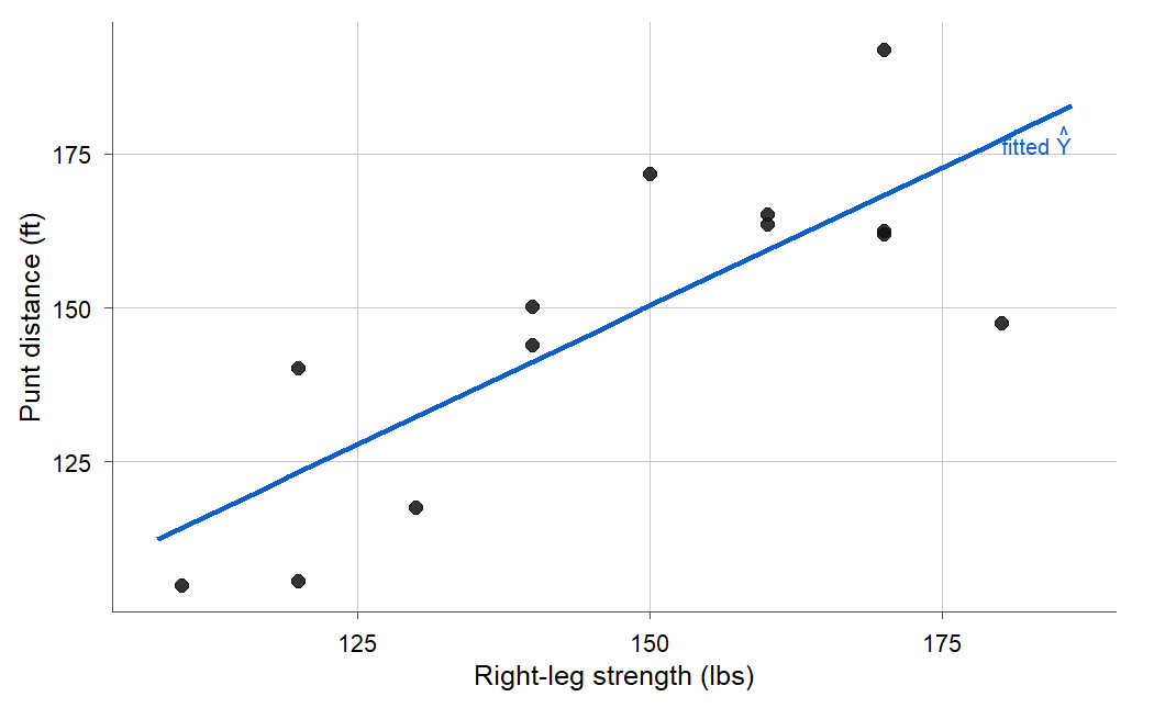
Figure 1:The thirteen punters, with the least-squares line. Distance climbs with right-leg strength at about 0.9 feet per pound, but thirteen points make it fair to ask whether the slope is real or an accident of a small sample.
This chapter answers the question a different way. Instead of assuming a shape for the errors, it uses the computer to shuffle and resample the data thousands of times and watches what happens. Two ideas do the work. A permutation test (Definition 5.1) breaks the link between predictor and response by shuffling, then asks how often pure chance produces a slope as steep as the one you saw. The bootstrap (Definition 5.4) resamples the data with replacement to see how much the slope would bounce around if you could collect the study again. Both replace a fragile assumption with a computation you can always run. By the end you will be able to build each one from scratch, read its output, and say when it agrees with the classical and tests and when it does not.
5.1 When normal-theory inference is on thin ice
Intuition
Every test from Chapter 3 came with fine print. Its formulas give exact answers only when the errors follow a normal bell curve, or when the sample is large enough to stand in for that. With thirteen punters we have neither, and this section shows that we cannot even check the fine print. Here is that fine print written out in symbols.
Chapter 3 built a confidence interval for the slope as and tested with the ratio , comparing it to a distribution with degrees of freedom. That machinery is exact only when the errors are normal. When they are not normal, the ratio is still approximately -distributed if the sample is large, because a version of the central limit theorem smooths the estimate toward normality. The catch is the word large. With thirteen punters there is no large-sample rescue, and there is no way to confirm the errors are normal.
You might think you could just check: fit the line, plot the thirteen residuals on a normal quantile plot, and see whether they fall on a straight line. The problem is that thirteen points are too few to tell normal from non-normal. Figure 2 makes this concrete. The top-left panel is the real punting residuals; the other five are genuinely normal samples of the same size, drawn by the computer. Every one of them bends and wiggles away from the straight line. If known-normal data looks this crooked at , then a crooked plot from real data tells you almost nothing. The normality assumption is simply uncheckable here.
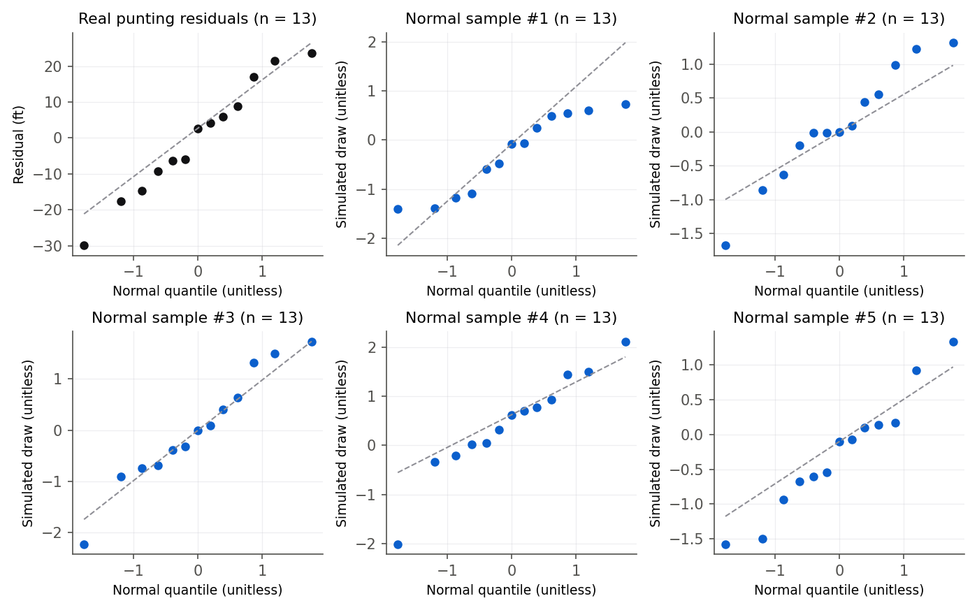
Figure 2:At n = 13 even data that is genuinely normal (the five blue panels) produces a bent, wandering quantile plot. So the crooked plot of the real residuals (top left) is no evidence against normality: thirteen points cannot tell the two apart. This is why we want inference that does not lean on a normality check.
The way out is to stop assuming a distribution and start generating one. If we can build the distribution of the slope under some clearly stated chance mechanism, using only the data in hand, then we can measure how surprising the observed slope is without ever writing down a normal density. That is what the rest of the chapter does.
5.2 The permutation test for the slope
Intuition
Here is the question a hypothesis test asks, in plain words: if leg strength had nothing to do with punt distance, how often would random chance hand us a slope as steep as 0.902? To answer it we need to see slopes produced by “nothing going on.” We can manufacture them. Keep the thirteen strength values exactly where they are, take the thirteen distances, and shuffle them so that each distance is reassigned to a random punter. Shuffling destroys any real link between strength and distance while keeping both columns of numbers intact. Fit a line to the shuffled data and record its slope. That slope is a sample of “what a slope looks like when there is no association.”
Figure 3 shows one shuffle. On the left, the real data slopes up. On the right, the same distances reattached to random strengths give a nearly flat line. Do the shuffle thousands of times and you get thousands of no-association slopes: their histogram is the null distribution of the slope, built entirely from your own data with no formula and no normality assumption.
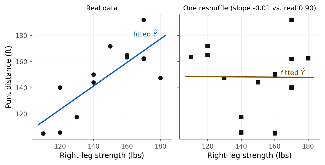
Figure 3:Shuffling the distances against the fixed strengths breaks the link between them, so a reshuffled fit has a slope near zero. Repeating the shuffle thousands of times shows what slopes chance alone can produce.
Formula
The permutation test for the slope works with these pieces. Let the data be pairs for , and let the observed least-squares slope be
In words: the slope is the cross-product of and deviations divided by the spread of , exactly as in 2.2 Least squares from first principles. The null hypothesis is
and the alternative is that they are related (). A permutation is a reshuffling of the response values that pairs with . For each permutation compute the reshuffled slope . The two-sided permutation p-value is the fraction of permutations whose slope is at least as far from zero as the observed one:
In words: the p-value is how often a reshuffle beats or ties the real slope in size, plus one for the real data itself, divided by the number of tries plus one. There are possible permutations, far too many to list ( is over six billion), so we draw of them at random and use those. The extra +1 on top and bottom counts the observed arrangement as one of the possibilities, which we explain and justify next.
Derivation (why the permutation test is valid)
Proof. Suppose holds in the strong sense that the response values were attached to the predictor values without any regard to them. Then the particular pairing we observed is just one of the equally likely ways to match the fixed collection of values to the fixed values. Any statistic computed on a random pairing, here the slope , therefore has a completely known distribution under : it places probability on each of the arrangements. This is the permutation distribution, and it needs no assumption about the shape of the errors. Normality never appears.
Our observed slope is the value from one particular arrangement, so under it is one draw from that permutation distribution. The exact two-sided p-value is the null probability of a slope at least as extreme in size,
which counts arrangements, including the observed one (it satisfies with equality). When is too large to enumerate, we estimate by drawing random permutations. Writing for the number of those draws with , the estimator
adds the observed arrangement to both the count and the total. This +1 is not a fudge. It keeps the test honest: the observed data is itself a valid arrangement under , so it belongs in the reference set, and including it guarantees can never be exactly zero. A test that could report would reject with certainty on finite evidence, which is never justified. With the +1, the smallest possible p-value is , and one can show the resulting test never rejects a true null more often than its stated level.
One tidy consequence: because and the do not change when we shuffle , the reshuffled slope is just , a fixed positive constant times the reshuffled cross-product . So permuting the slope is the same test as permuting the sample correlation, or permuting itself. Whatever monotone version of “association” you prefer, the permutation test gives the same p-value.
R
The permutation test is a short loop. Read the data, write a one-line slope function, compute the observed slope, then shuffle and refit times. No package beyond base R is needed.
punting <- read.csv("data/punting.csv")
dim(punting)
fit <- lm(Distance ~ RStr, data = punting)
round(summary(fit)$coefficients, 5)
[1] 13 7
Estimate Std. Error t value Pr(>|t|)
(Intercept) 15.00896 31.35922 0.47861 0.64159
RStr 0.90204 0.21003 4.29474 0.00127The classical fit gives a slope of 0.902 feet per pound with a -test p-value of 0.00127. Hold on to that number; the permutation test will produce its own p-value to compare against it. Now the from-scratch pieces.
slope <- function(x, y) {
  sum((x - mean(x)) * (y - mean(y))) / sum((x - mean(x))^2)
}
x <- punting$RStr
y <- punting$Distance
b1_obs <- slope(x, y)
b1_obs
[1] 0.9020383set.seed(4210)
B <- 5000
perm_slopes <- numeric(B)
for (i in 1:B) {
y_shuffled <- sample(y) # shuffle distances, keep strengths fixed
perm_slopes[i] <- slope(x, y_shuffled)
}
count_extreme <- sum(abs(perm_slopes) >= abs(b1_obs))
p_perm <- (count_extreme + 1) / (B + 1)
c(count_extreme = count_extreme, p_permutation = p_perm)count_extreme p_permutation
4.0000000 0.0009998 Out of 5000 reshuffles, only 4 produced a slope as steep as the real one, so the permutation p-value is .
Python
The same loop in Python with NumPy. rng.permutation does the shuffling; everything else is a
handful of array operations.
import numpy as np
import pandas as pd
import statsmodels.formula.api as smf

punting = pd.read_csv("data/punting.csv")
print(punting.shape)
fit = smf.ols("Distance ~ RStr", data=punting).fit()
print(fit.summary().tables[1])
(13, 7)
==============================================================================
coef std err t P>|t| [0.025 0.975]
------------------------------------------------------------------------------
Intercept 15.0090 31.359 0.479 0.642 -54.012 84.030
RStr 0.9020 0.210 4.295 0.001 0.440 1.364
==============================================================================def slope(x, y):
x = np.asarray(x, float)
y = np.asarray(y, float)
return np.sum((x - x.mean()) * (y - y.mean())) / np.sum((x - x.mean()) ** 2)
x = punting["RStr"].to_numpy()
y = punting["Distance"].to_numpy()
b1_obs = slope(x, y)
print(b1_obs)0.9020382716049381rng = np.random.default_rng(4210)
B = 5000
perm_slopes = np.empty(B)
for i in range(B):
y_shuffled = rng.permutation(y) # shuffle distances, keep strengths fixed
perm_slopes[i] = slope(x, y_shuffled)
count_extreme = int(np.sum(np.abs(perm_slopes) >= abs(b1_obs)))
p_perm = (count_extreme + 1) / (B + 1)
print("count_extreme =", count_extreme, " p_permutation =", p_perm)count_extreme = 5 p_permutation = 0.0011997600479904018R and Python use different random number generators, so they draw different shuffles: R found 4 extreme slopes and Python found 5, giving permutation p-values of about 0.0010 and 0.0012. The two disagree only in the third decimal place, which is Monte Carlo noise, and both point to the same clear conclusion.
The permutation test is easier to believe once you have watched chance produce a few hundred slopes yourself and seen where 0.902 lands among them, so run the shuffling before moving on.
Shuffle the thirteen punt distances against the fixed strengths, refit each time, and watch the no-association null distribution of the slope build up underneath the observed 0.902.
What to notice. Every shuffle keeps the same thirteen strengths and the same thirteen distances, so the only thing that changed is which distance went with which punter. Try this. Press Run 1000 three times, read off the readout, then compute by hand and check it against the p-value the widget reports (5.2 The permutation test for the slope).
5.3 Permutation on Toluca, and how it compares with the t test
The punting example ended in a near-tie between the permutation and -test p-values. To see the two methods on a case where the signal is overwhelming, return to the Toluca Company data from Chapters 2 and 3: the labor hours to produce a part against the lot size, with the least-squares slope hours per unit (2.2 Least squares from first principles). Chapter 3 tested that slope with a test and found a p-value of about (3.7 The F test and its equivalence to the t test, where the and tests coincide for a single slope). We now run the permutation test on the same slope and compare.
toluca <- read.csv("data/toluca.csv")
xt <- toluca$lotsize
yt <- toluca$hours
b1_toluca <- slope(xt, yt)
p_t <- summary(lm(hours ~ lotsize, data = toluca))$coefficients["lotsize", "Pr(>|t|)"]

set.seed(4210)
perm_toluca <- numeric(B)
for (i in 1:B) perm_toluca[i] <- slope(xt, sample(yt))
c(b1_toluca      = b1_toluca,
  perm_count     = sum(abs(perm_toluca) >= abs(b1_toluca)),
  max_perm_slope = max(abs(perm_toluca)),
  t_test_p_value = p_t)
b1_toluca perm_count max_perm_slope t_test_p_value
3.570202e+00 0.000000e+00 2.767172e+00 4.448828e-10 toluca = pd.read_csv("data/toluca.csv")
xt = toluca["lotsize"].to_numpy()
yt = toluca["hours"].to_numpy()
b1_toluca = slope(xt, yt)
p_t = smf.ols("hours ~ lotsize", data=toluca).fit().pvalues["lotsize"]
rng = np.random.default_rng(4210)
perm_toluca = np.array([slope(xt, rng.permutation(yt)) for _ in range(B)])
print("b1_toluca =", b1_toluca)
print("perm_count =", int(np.sum(np.abs(perm_toluca) >= abs(b1_toluca))))
print("max_perm_slope =", np.max(np.abs(perm_toluca)))
print("t_test_p_value =", p_t)b1_toluca = 3.57020202020202
perm_count = 0
max_perm_slope = 2.7454545454545456
t_test_p_value = 4.4488275871889375e-10The floor raises a fair question: how many reshuffles is enough? Because is a Monte Carlo estimate, it wobbles from run to run when is small and settles as grows. Figure 7 tracks the running punting p-value against the number of reshuffles used, for three different random seeds. Past a few thousand reshuffles the three lines have nearly stopped moving, which is why this chapter uses . If you needed to resolve a p-value near a sharp cutoff, you would run more.
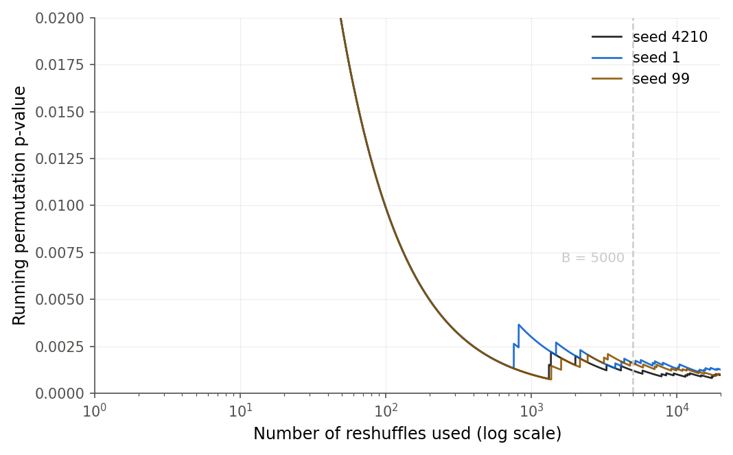
Figure 7:The running punting permutation p-value for three random seeds. Each estimate is noisy for the first few hundred reshuffles and settles near 0.001 by a few thousand, the reason B = 5000 is a reasonable default.
5.4 The bootstrap for regression
Intuition
A permutation test answers “is there an effect?” It does not tell you how big the effect is or how precise your estimate of it is. For that we want the sampling distribution of : the spread of slopes you would see if you could repeat the whole study many times. We cannot repeat the study. The bootstrap fakes the repetition using the one sample we have, by resampling it with replacement. The idea, due to Bradley Efron, is that the sample is our best picture of the population, so drawing new samples from the sample imitates drawing new samples from the population.
There are two natural ways to resample a regression, and they answer slightly different questions. Figure 8 shows both. Case resampling draws whole rows with replacement, so a given punter may appear twice or not at all, and the set of strength values changes from resample to resample. This treats the punters as a random sample from a population of punters. Residual resampling keeps the strengths and the fitted line fixed, then builds a new response by adding reshuffled-with-replacement residuals back onto the fitted values. This treats the strength values as fixed by design and puts all the randomness in the errors, matching the regression model of Chapter 2 more literally.
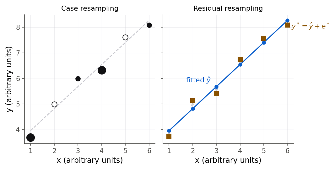
Figure 8:The two bootstraps for regression. Case resampling (left) redraws whole rows, so which x-values appear changes each time. Residual resampling (right) keeps the x-values and the fitted line fixed and reattaches reshuffled residuals, putting all the randomness in the errors.
Formula
Both bootstraps repeat a resample-and-refit loop times and collect the slopes. The case-resampling algorithm is:
In words: rebuild a dataset by drawing rows at random with repeats allowed, and refit. The residual-resampling algorithm fixes and the observed fit with residuals :
where is a residual drawn at random with replacement from . In words: keep the line and the strengths, then jiggle each fitted point up or down by a residual borrowed from somewhere in the data. The bootstrap standard error of the slope is the standard deviation of the collected slopes,
the ordinary spread of the resampled slopes. It estimates how much would vary across repeated studies.
R
Case resampling is a loop that resamples row indices. We reuse the slope function from before.
set.seed(4210)
n <- nrow(punting)
boot_case <- numeric(B)
for (i in 1:B) {
  idx <- sample(n, n, replace = TRUE)  # resample whole rows
  boot_case[i] <- slope(x[idx], y[idx])
}
c(boot_mean = mean(boot_case), boot_SE = sd(boot_case))
boot_mean boot_SE
0.9045003 0.2485204 Residual resampling keeps x fixed and rebuilds y from the fitted values plus resampled
residuals.
b0_obs <- mean(y) - b1_obs * mean(x)
fitted_vals <- b0_obs + b1_obs * x
resid_obs <- y - fitted_vals

set.seed(4210)
boot_resid <- numeric(B)
for (i in 1:B) {
  y_star <- fitted_vals + sample(resid_obs, n, replace = TRUE)
  boot_resid[i] <- slope(x, y_star)
}
c(boot_mean = mean(boot_resid), boot_SE = sd(boot_resid))
boot_mean boot_SE
0.9020770 0.1976297 Python
rng = np.random.default_rng(4210)
n = len(punting)
boot_case = np.empty(B)
for i in range(B):
    idx = rng.integers(0, n, n)           # resample whole rows
    boot_case[i] = slope(x[idx], y[idx])
print("boot_mean =", boot_case.mean(), " boot_SE =", boot_case.std(ddof=1))
boot_mean = 0.9099216280489136 boot_SE = 0.24681912512413196b0_obs = y.mean() - b1_obs * x.mean()
fitted_vals = b0_obs + b1_obs * x
resid_obs = y - fitted_vals
rng = np.random.default_rng(4210)
boot_resid = np.empty(B)
for i in range(B):
y_star = fitted_vals + rng.choice(resid_obs, n, replace=True)
boot_resid[i] = slope(x, y_star)
print("boot_mean =", boot_resid.mean(), " boot_SE =", boot_resid.std(ddof=1))boot_mean = 0.9009502801536351 boot_SE = 0.1951940681246211The case bootstrap is a loop of four lines, but the picture of punters appearing twice and vanishing is what makes the standard error stop being a formula, so redraw a few resamples by hand.
Resample the thirteen punters with replacement, refit, and watch the bootstrap distribution of the slope build up around the observed 0.902 rather than around zero.
What to notice. Put this histogram next to the permutation one: the null pile sits on zero because shuffling destroyed the effect, while the bootstrap pile sits on because resampling preserves it. Try this. Run 1000 three times and compare the bootstrap standard error against the formula’s 0.210, then explain the gap using the changing set of strengths (5.4 The bootstrap for regression).
5.5 Bootstrap confidence intervals
Intuition
A standard error is a single number for the spread. A confidence interval is a range that should contain the true slope with, say, confidence. The bootstrap distribution of the slope already contains the information; we just have to read an interval off it. Two simple recipes do this without assuming the distribution is normal (both are collected in Definition 5.7). The percentile interval takes the middle of the bootstrap slopes directly. The basic interval (also called the reflection interval) corrects for a subtle bias by flipping the percentiles around the observed slope. When the bootstrap distribution is symmetric they nearly coincide; when it is skewed they part ways, and the basic interval is usually the better behaved of the two.
Formula
Let and be the lower and upper percentiles of the bootstrap slopes, for a interval (so for ). The two intervals are
In words: the percentile interval is just the 2.5th and 97.5th percentiles of the resampled slopes; the basic interval reflects those two percentiles through twice the observed slope. Notice the basic interval swaps the roles of the two percentiles, because reflecting turns the upper tail into the lower endpoint.
That swap is easier to see than to say. Figure 11 draws it. Think of the observed slope as a mirror standing in the middle. The percentile interval sits above; to get the basic interval you reflect each endpoint through the mirror, so the point that was far to the right lands far to the left and vice versa. The arithmetic is exactly “reflect across ”: it measures how far sits from and steps the same distance to the other side.
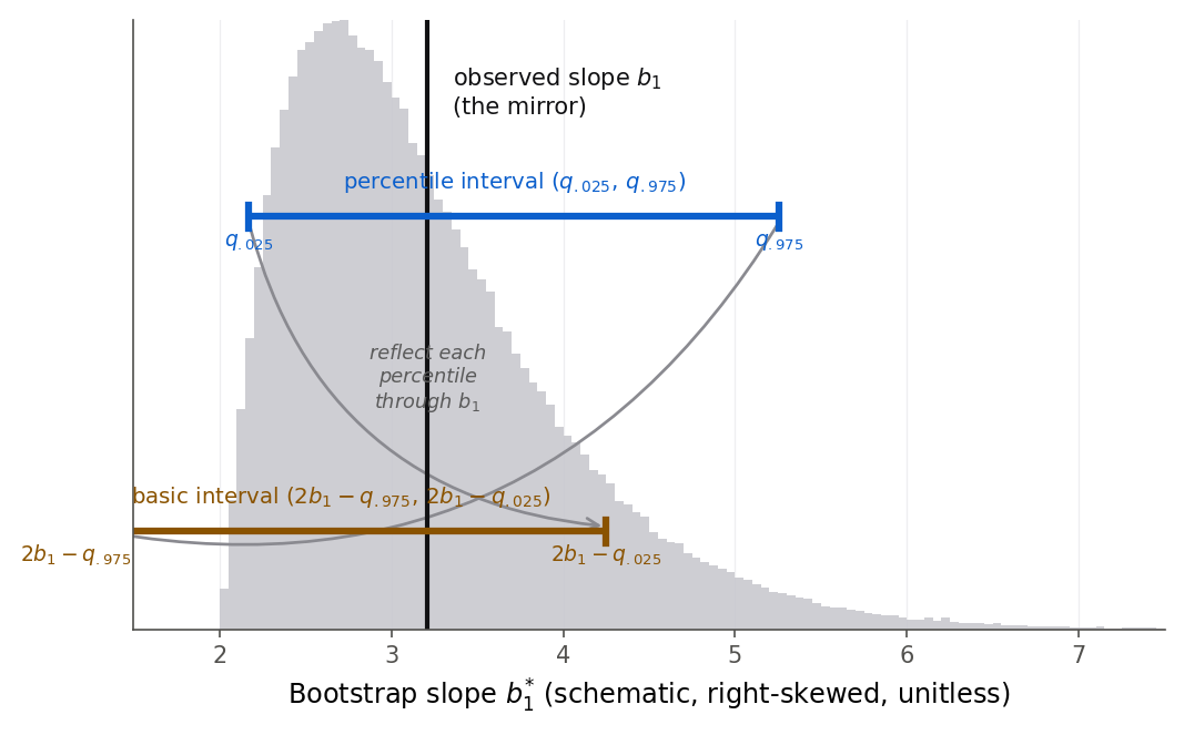
Figure 11:The basic interval is the percentile interval mirrored through the observed slope b1. Reflecting swaps the tails: the far-right percentile becomes the left endpoint and the far-left percentile becomes the right endpoint. On a skewed distribution like this one the two intervals sit in different places; on a symmetric one they land on top of each other.
Derivation (the basic bootstrap interval)
Proof. The bootstrap principle says the variation of the resampled slope around the observed slope imitates the variation of the observed slope around the true slope. Write this as: the distribution of approximates the distribution of . Let and be the percentiles of , so by definition
Subtract throughout to center on the observed slope:
Now use the bootstrap principle to replace with , which has approximately the same distribution:
Solve the inequalities for . Subtracting and negating (which flips the inequality directions and swaps the endpoints) gives
That bracket is the basic interval. The percentile interval is what you get if you skip the pivoting step and read the bootstrap percentiles as if they were percentiles of directly. The two agree exactly when the bootstrap distribution is symmetric about , because then reflecting the percentiles through lands them back on themselves.
R
perc_ci  <- quantile(boot_case, c(0.025, 0.975))
basic_ci <- c(2 * b1_obs - perc_ci[[2]], 2 * b1_obs - perc_ci[[1]])
t_ci     <- confint(fit)["RStr", ]
round(c(perc_lo = perc_ci[[1]], perc_hi = perc_ci[[2]]), 4)
round(c(basic_lo = basic_ci[1], basic_hi = basic_ci[2]), 4)
round(c(t_lo = t_ci[[1]], t_hi = t_ci[[2]]), 4)
perc_lo perc_hi
0.4158 1.3883
basic_lo basic_hi
0.4158 1.3883
t_lo t_hi
0.4398 1.3643 Python
perc_ci = np.quantile(boot_case, [0.025, 0.975])
basic_ci = np.array([2 * b1_obs - perc_ci[1], 2 * b1_obs - perc_ci[0]])
t_ci = fit.conf_int().loc["RStr"].to_numpy()
print("percentile", np.round(perc_ci, 4))
print("basic     ", np.round(basic_ci, 4))
print("classical ", np.round(t_ci, 4))
percentile [0.413 1.3824]
basic [0.4216 1.3911]
classical [0.4398 1.3643]Figure 11 is a still photograph of the reflection. The widget below is the same picture with a handle on it: you can skew the bootstrap distribution yourself and watch the two intervals come apart.
Move one punter to skew the case-bootstrap distribution of the slope, and watch the percentile interval and its reflection through b1, the basic interval, separate.
What to notice. The two bars coincide only while the bootstrap pile is symmetric about the mirror at ; skew is exactly what pulls them apart. Try this. Drag the strongest punter down to 100 feet, then check the reported endpoints against and with a calculator (5.5 Bootstrap confidence intervals).
5.6 When computational and classical inference agree
You have now met every tool in the chapter. Before comparing their answers, it helps to see them on one page. Figure 14 is a map: it starts from your fitted slope and asks what you want to know, then walks you to the right method. The first fork is the big one. If you want to know whether an effect exists at all, you run a permutation test and report a p-value. If you want to know how precise your estimate is, you run a bootstrap and report a standard error or confidence interval. The bootstrap then forks again by how the data were collected: case resampling for randomly sampled subjects, residual resampling for a design with fixed predictor values.
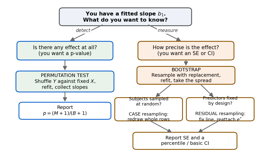
Figure 14:The chapter on one page. The first question, detect an effect or measure its precision, chooses between the permutation test and the bootstrap; the bootstrap then splits by how the data arose.
You have now seen three verdicts on the punting slope (permutation, bootstrap, classical) that all pointed the same way, and a Toluca slope where they agreed up to the permutation test’s resolution floor. That is the common case: when the classical assumptions roughly hold, the computational and classical answers match, and the agreement is itself evidence that the classical p-value can be trusted. The methods earn their keep when the assumptions are shaky, because then the resampling answer does not depend on those assumptions.
To see the agreement directly, compare the bootstrap and classical standard errors on the Toluca slope, where and the data are clean.
set.seed(4210)
boot_toluca <- numeric(B)
nt <- length(xt)
for (i in 1:B) {
  idx <- sample(nt, nt, replace = TRUE)
  boot_toluca[i] <- slope(xt[idx], yt[idx])
}
classical_se <- summary(lm(hours ~ lotsize, data = toluca))$coefficients["lotsize", "Std. Error"]
c(bootstrap_SE = sd(boot_toluca), classical_SE = classical_se)
bootstrap_SE classical_SE
0.3765516 0.3469722 rng = np.random.default_rng(4210)
nt = len(xt)
boot_toluca = np.empty(B)
for i in range(B):
idx = rng.integers(0, nt, nt)
boot_toluca[i] = slope(xt[idx], yt[idx])
classical_se = smf.ols("hours ~ lotsize", data=toluca).fit().bse["lotsize"]
print("bootstrap_SE =", boot_toluca.std(ddof=1), " classical_SE =", classical_se)bootstrap_SE = 0.36568568108182364 classical_SE = 0.3469721568487608A wrong reading to avoid: a student sees the bootstrap standard error 0.377 next to the classical 0.347 and concludes “the bootstrap is wrong, because it does not match the formula.” That gets it backward. Neither number is the truth; both estimate the same unknown standard deviation of , and they differ only by sampling noise and by the small extra variability case resampling includes on purpose. The right reading is that they agree well enough to reinforce each other. You would only worry if they disagreed by a lot, which would be a signal that the classical assumptions are failing and the bootstrap is telling you something the formula cannot.
5.7 Chapter summary
You can now do inference for a regression slope without leaning on the normal error assumption. When a small sample puts the and tests on thin ice and thirteen residuals cannot confirm normality, you replace the untestable assumption with a computation. A permutation test shuffles the response against the fixed predictor to build the no-association null of the slope and reports ; on the punting data it gave , matching the classical 0.00127. A bootstrap resamples the data with replacement to measure precision: case resampling and residual resampling gave slope standard errors of about 0.249 and 0.198, and percentile and basic intervals near , all consistent with the classical . The recurring lesson is that when computational and classical answers agree the agreement builds trust, and when they diverge sharply that divergence is a warning about assumptions.
Key results at a glance.
| Result | Statement or formula | Valid when |
|---|---|---|
| Permutation test (Definition 5.1) | Shuffle against fixed , refit, collect slopes | No-association null; any error distribution |
| Permutation p-value (Definition 5.2) | of reshuffles at least as extreme | |
| Validity of the permutation p-value (Theorem 5.3) | ; floor | Under the no-association null |
| Bootstrap (Definition 5.4) | Resample with replacement, recompute, take the spread | Sample stands in for the population |
| Case vs residual resampling (Definition 5.5) | Rows with replacement, or | Random subjects, or fixed-design predictor |
| Bootstrap standard error (Definition 5.6) | resamples of the fitted model | |
| Percentile / basic intervals (Definition 5.7) | / | Read off the bootstrap distribution |
| Basic interval by pivoting (Theorem 5.8) | Reflect percentiles through ; equals percentile if symmetric | Bootstrap principle holds |
Key terms. Permutation test, permutation distribution, permutation p-value, plus-one correction, bootstrap, case resampling, residual resampling, bootstrap standard error, percentile interval, basic bootstrap interval, exchangeability.
You should now be able to.
Explain why normal-theory and inference for a slope can fail, and why a small sample makes the risk worse and normality uncheckable.
State the no-association null and describe the exact logic of a permutation test for the slope.
Implement the permutation test from scratch in R and Python and compute a permutation p-value.
Justify the plus-one correction and the resolution floor , and compare against the classical -test p-value.
Distinguish case resampling from residual resampling and code each one.
Construct and interpret percentile and basic bootstrap confidence intervals for the slope.
Decide when computational and classical inference agree, and what to report when they disagree.
Where this fits. On the workflow spine of The modeling workflow, this chapter lives in USE: it is inference, turning a fitted slope into a defensible statement about the world. It is also a quiet CHECK, because comparing computational and classical answers audits the assumptions behind the classical ones. Chapter 3 gave the classical and inference that assumes normal errors; this chapter gave the resampling inference that does not, and showed the two agree when the assumptions hold. The bootstrap returns later as a working tool: Chapter 9 reaches for it when diagnostics say normality has failed, and Chapter 12 uses the same resample-and-refit mindset to validate models on data they were not fit to (12.4 Validation: train, test, and cross-validate). The habit you built here, generate the distribution instead of assuming it, is one you will use for the rest of the book.
5.8 Frequently asked questions
Q1. Is a permutation test the same as a bootstrap? No, though both resample. A permutation test shuffles without replacement to break the link between and , building the distribution of a statistic under the null hypothesis of no association; it answers “is there an effect?” The bootstrap resamples with replacement to imitate repeated sampling from the population, building the distribution of the estimate itself; it answers “how precise is the effect?” Use a permutation test for a p-value, a bootstrap for a standard error or confidence interval.
Q2. Why shuffle without replacement for the permutation test but with replacement for the bootstrap? The permutation test needs every reshuffle to be a genuine rearrangement of the same values, so that it represents one of the equally likely pairings under the null; sampling without replacement (a shuffle) does exactly that. The bootstrap needs each resample to look like a fresh draw from the population, and real repeated samples can contain repeats and omissions, so it samples with replacement.
Q3. How many reshuffles or resamples do I need? Enough that the answer stops moving. For a p-value you are comparing to 0.05, a few thousand reshuffles is usually plenty; near a sharp cutoff, use more, because the Monte Carlo floor is and the noise shrinks like . For a bootstrap standard error, 1000 to 2000 resamples often suffice; for the tail percentiles of a confidence interval, use 5000 or more, since the extreme quantiles are noisier than the center.
Q4. My permutation p-value is 0. Do I report ? Never report exactly zero. If no reshuffle out of beat your statistic, the plus-one correction gives , and you report “less than” that: for , report . Reporting would claim infinite certainty from finite data.
Q5. Which bootstrap should I use, case or residual? Match the resampling to how the data arose. If the predictor values were fixed by design (a planned experiment with set doses, or the Toluca lot sizes chosen by schedulers), residual resampling fits the model literally. If the rows are a random sample from a population and the predictor is just another measured variable (the punters), case resampling is more honest. It is also the safer default when you are unsure, because it captures variability in the predictor and does not assume constant error variance.
Q6. The bootstrap and the test gave slightly different intervals. Which is right? Neither is “right” in an absolute sense; both estimate the same true uncertainty. When they are close, as in the punting and Toluca examples, trust either and note the agreement. When they differ a lot, the disagreement is information: it usually means a classical assumption (normality, constant variance, no influential points) is failing, and the assumption-free bootstrap is the safer report while you investigate.
Q7. Do these methods work for multiple regression? Yes. The bootstrap generalizes directly: case-resample whole rows, or residual-resample around the fitted surface, and collect whichever coefficient you care about. Permutation is subtler with several predictors, because shuffling one predictor while holding others fixed requires care about what null you are testing, but the core idea carries over. This chapter keeps to simple regression so the logic stays visible; the resampling code changes little when you add predictors.
5.9 Practice problems
(A) In one sentence each, state what question a permutation test answers and what question a bootstrap answers, and say which resamples with replacement.
(A) Explain why thirteen residuals cannot confirm or rule out normal errors, referring to Figure 2.
(A) State the null and alternative hypotheses of the permutation test for a slope, in words and in symbols.
(A) Why does the permutation p-value use the plus-one correction instead of ? What goes wrong if a test can report exactly zero?
(A) A permutation test with reshuffles finds . What p-value do you report, and what is the smallest p-value this run could ever give?
(A) Describe in words the difference between case resampling and residual resampling, and give one data-collection story that fits each.
(A) The percentile interval for a slope is and the observed slope is . Without a computer, find the basic interval.
(A) A classmate reports a permutation p-value of 0 for a slope. Rewrite their conclusion so it is defensible, assuming they used reshuffles.
(A) Explain why shuffling against fixed , shuffling against fixed , and shuffling both give the same permutation test.
(B) Show that when you permute the response, the reshuffled slope is a fixed positive constant times the reshuffled cross-product , and conclude that the permutation test on the slope is identical to the permutation test on the sample correlation.
(B) Derive the basic bootstrap interval (Theorem 5.8) from the bootstrap principle that has approximately the same distribution as . Show every step of the algebra that flips the endpoints.
(B) Prove that the percentile and basic intervals coincide exactly when the bootstrap distribution of is symmetric about .
(B) The exact two-sided permutation p-value counts arrangements with out of . Explain why the observed arrangement is always counted, and use this to argue that the exact p-value is at least .
(B) A statistic has permutation distribution placing probability on each arrangement. Explain why, under the null, the random variable (computed from the full enumeration) satisfies for any cutoff that is a multiple of , so the test controls its error rate (Theorem 5.3).
(B) The Monte Carlo standard error of a bootstrap standard-error estimate shrinks like . Explain qualitatively why doubling the accuracy of a tail confidence-interval endpoint costs four times the resamples.
(B) Explain why the case-bootstrap standard error can exceed the classical formula standard error even when the model is correct, by naming the extra source of variation case resampling includes that the residual bootstrap and the classical formula hold fixed.
(C) Reproduce the punting permutation test in R or Python with
set.seed(4210)/default_rng(4210)and . Report the count of extreme reshuffles and the permutation p-value, and compare to the classical -test p-value 0.00127.(C) Repeat the punting permutation test with the predictor
LStr(left-leg strength) instead ofRStr. Report the observed slope, the permutation p-value, and whether your conclusion changes.(C) Run the Toluca permutation test with . Report the largest reshuffled slope in size and explain why the permutation p-value cannot go below here.
(C) Compute the case-bootstrap and residual-bootstrap standard errors of the punting slope with . Report both and explain which is larger and why.
(C) Compute percentile and basic intervals for the punting slope from the case bootstrap, and put them next to the classical interval . Comment on the agreement.
(C) Using the
puntingdata and predictorOStr(overall leg strength), build a percentile bootstrap interval for the slope (use the 5th and 95th percentiles). Report the interval and interpret it in the units of the problem.(C) Bootstrap the Toluca slope 5000 times by case resampling and compare the bootstrap standard error to the classical 0.347. State the percentage difference and whether the two agree.
(C) Write a permutation test for the punting slope but use the sample correlation as the statistic instead of the slope. Confirm that the p-value matches the slope-based test (problem 17), illustrating the identity from problem 10.
(C) Increase the punting permutation test to reshuffles. Does the p-value estimate change materially from the value? Report both and comment on Monte Carlo noise.
(C) Make a normal quantile plot of the punting residuals in R or Python, then generate three normal samples of size 13 and plot their quantile plots. Describe how hard it is to tell the real residuals from the normal samples, connecting to Figure 2.
(C) For the punting slope, compute a bootstrap standard error and form the interval (a normal-approximation bootstrap interval). Compare it to the percentile interval and explain when the two would disagree.
(B) An analyst uses a paired shuffle: they reorder the rows of the data but keep each pair together, then refit. Show that every such “permutation” gives exactly the observed slope, and explain why this tests nothing.
5.10 Exam practice
These five questions match the style of the course exams: each one asks you to explain, evaluate, or interpret in full sentences, not just to compute a number. Write your own answer before opening the model answer. A correct number with no reasoning would earn little credit on the real exam, and a clear explanation with a small arithmetic slip would earn most of it.
EP 5.1 (explain why). The chapter calls the classical test for the punting slope “on thin ice” with , yet it runs the permutation test on those same thirteen punters without apology. Explain, in full sentences, exactly which assumption the test needs that the permutation test does not, and why having only thirteen punters makes that difference matter here instead of being a technicality.
Model answer
The classical test treats the ratio as exactly -distributed on degrees of freedom, and that distribution is exact only when the errors are normal. When the errors are not normal, the result holds only as an approximation, and only when the sample is large enough for a central-limit effect to smooth the slope estimate toward normality. With thirteen punters there is no large-sample rescue, and thirteen residuals cannot tell a normal distribution from a non-normal one (Figure 2), so the single premise the test leans on is precisely the one that cannot be checked. That is what “thin ice” means: not that the test is known to be wrong, but that its safety net is unverifiable.
The permutation test needs no distributional assumption at all. Under the no-association null the thirteen distances are attached to the thirteen strengths without regard to them, so the observed slope is literally one of the equally likely pairings, and reshuffling generates that reference distribution exactly from the data in hand. Normality never enters the argument, so the small sample that undermines the test does not undermine the permutation test. The only price the permutation test pays for small is a coarser reference set (fewer genuinely distinct pairings), not a broken assumption.
A weak answer just says “permutation tests do not assume normality” without explaining that the test’s normality requirement is exactly the uncheckable one at , and without noting that the permutation reference distribution comes from the equally likely pairings under the null.
EP 5.2 (interpret output and a figure in context). A different physical test, hang time (the
seconds the ball stays airborne), is used to predict punt distance with the model
Distance ~ Hang. The classical fit and a permutation test with (seed 4210) give:
Distance ~ Hang
             Estimate Std. Error  t value Pr(>|t|)
(Intercept) -22.32579   36.30608 -0.61493  0.55111
Hang         43.50138    9.19420  4.73139  0.00062

permutation test: 2 of 5000 reshuffles as extreme,  p_perm = (2+1)/(5000+1) = 0.0006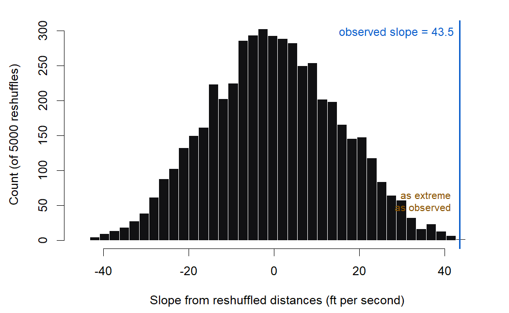
Figure 15:The permutation null distribution of the hang-time slope. Reshuffled slopes cluster around zero; the observed slope 43.5 sits off the right edge, beaten by only two of 5000 reshuffles, so the two-sided permutation p-value is about 0.0006.
Interpret this output and figure in context. State what the slope 43.5 means in the units of the problem, what the two p-values say and whether they agree, and give one sentence of caution about what this analysis does not establish.
Model answer
The slope says that among these thirteen punters, each additional second of hang time goes with about 43.5 more feet of average punt distance. The intercept -22.3 feet is not interpretable on its own, because a hang time of zero is far outside the range of the data and would mean the ball never left the foot. Both p-values are tiny and essentially identical: the classical test gives 0.00062 and the permutation test gives . The figure shows why they agree, because the observed slope 43.5 sits off the far right edge of the reshuffled null, beaten by only two of five thousand shuffles. So a slope this steep almost never arises when hang time and distance are unrelated, and we have strong evidence that the two are associated, a conclusion that does not lean on normal errors because the assumption-free permutation test lands in the same place as the test.
The caution: this is an observational association measured within thirteen punters, not a causal effect. It does not show that a punter could lengthen a kick by deliberately keeping the ball in the air longer, because hang time and distance are both downstream of the same leg strength and technique, and with only thirteen points the estimate 43.5 is itself imprecise.
A weak answer reads the p-value as “significant” but fails to interpret the slope in the units of the problem, does not note that the two methods agree and why that agreement matters, or slides into a causal claim.
EP 5.3 (a student claims something, evaluate it). A student runs the punting permutation test
(Distance ~ RStr, ) twice, once with set.seed(4210) and once with set.seed(2026),
and gets:
seed 4210:  M = 4 extreme reshuffles,  p_perm = 0.00100
seed 2026:  M = 8 extreme reshuffles,  p_perm = 0.00180
The student concludes: “The permutation test is unreliable, because it gives a different answer every time I run it. I should just report the classical test’s p-value of 0.00127, which is exact and reproducible.” Evaluate the student’s reasoning. Say what is right and what is wrong in each half of the claim.
Model answer
The student is half right and half wrong. It is true that a Monte Carlo permutation p-value wobbles from run to run, because it estimates the true permutation p-value from a finite random sample of reshuffles. The values 0.00100 and 0.00180 are two such estimates, and the gap between them is ordinary Monte Carlo noise, which shrinks like and would nearly disappear if the student ran far more reshuffles or enumerated all pairings. But “different every time” is not the same as “unreliable.” Both runs place the p-value near 0.001, both are far below any usual cutoff, and both lead to exactly the same decision, so the conclusion is not in doubt. The reproducibility worry is also already solved by fixing the seed, which the student did.
The second half of the claim is where the reasoning fails. The classical 0.00127 is “exact” only if its normality assumption holds, and the whole reason the chapter uses the punting data is that thirteen residuals cannot confirm normality. So that number is not more trustworthy than the permutation p-value, only more precise-looking. The honest report is the permutation p-value (about 0.001) together with the note that it agrees with the test, or a permutation run with a larger if a sharper figure is wanted.
A weak answer says only “it is random, so that is fine” without naming Monte Carlo error, the rate, or the fact that both runs give the same decision, and it fails to challenge the false claim that the test’s p-value is exact here.
EP 5.4 (a student claims something, evaluate it). The chapter’s RStr example found the
case-bootstrap standard error (0.249) larger than the residual-bootstrap one (0.198), and
explained that case resampling “adds one more source of variability.” A student turns this into a
rule: “Case resampling always gives a larger standard error than residual resampling, because it
lets the predictor values vary too.” To test the rule they refit punt distance on overall leg
strength (OStr) with and get:
Distance ~ OStr
classical formula standard error   = 0.0991
case-resampling bootstrap SE       = 0.0889
residual-resampling bootstrap SE   = 0.0910
Evaluate the student’s rule in light of this output.
Model answer
The rule is false as stated, and this output is a clean counterexample. Here the case-bootstrap
standard error (0.089) is actually smaller than the residual-bootstrap one (0.091), the reverse
of the RStr pattern. The chapter’s explanation described a tendency, not a guarantee. Case
resampling and residual resampling estimate the same underlying sampling variability of the slope by
two different mechanisms, and which one comes out larger on any given dataset depends on the
particular residuals and high-leverage points that happen to get resampled, plus ordinary Monte
Carlo noise. With only thirteen points these accidents easily swamp the “extra source of variation”
argument.
The sound reading is that the three standard errors (0.089, 0.091, and 0.099) all agree to within about ten percent and tell the same story about a slope of 0.43, so the choice between the two bootstraps should be made on the data-collection story (case resampling when the punters are a random sample from a population, residual resampling when the strengths are treated as fixed by design), not on which one happens to yield the bigger number.
A weak answer simply declares the rule right or wrong without using the printed numbers to show that case is smaller than residual here, or without explaining that the “extra variation” effect is only a tendency that small-sample noise can reverse.
EP 5.5 (what would change if). For the punting slope Distance ~ RStr (observed
), answer each part in full sentences.
(a) The chapter uses reshuffles and reports . What would change about the number you could honestly report if you reran the permutation test with only reshuffles and again found no reshuffle beating the observed slope?
(b) The chapter case-resamples the punters because they are treated as a sample from a larger population of punters. What would change about which bootstrap is the honest choice if instead these thirteen were the entire group you cared about, say the complete roster of one team, and you only wanted to describe the line within that fixed group?
Model answer
(a) With and , the permutation p-value would be , so the smallest number you could honestly report roughly doubles from the floor of . Fewer reshuffles raise the resolution floor , so you lose the ability to resolve very small p-values and your estimate is noisier from run to run, even though the qualitative conclusion (strong evidence, p well below 0.05) does not change. To report anything smaller you would have to run more reshuffles.
(b) If the thirteen punters are the whole group and you only want the line within that fixed set, the case for case resampling weakens. Case resampling imitates the randomness of drawing subjects from a population, and there is no such randomness left once you already have everyone. The variability worth modeling is then the scatter of the distances around the line, which is exactly what residual resampling captures by holding the strengths fixed and reattaching resampled residuals, so residual resampling (or the classical fixed-design view) becomes the more honest choice. In the extreme where the fit is treated as a pure description of one fixed finite group, inference about a wider population is arguably not even the right question to ask.
A weak answer to (a) misses that it is the floor that changes (about 0.002 versus 0.0002) rather than the decision; a weak answer to (b) just repeats “use case resampling” without recognizing that removing the sampling-of-subjects randomness removes the very reason to prefer it.
Chapter game
Resumen del capítulo (en español)
Este capítulo presenta la inferencia por remuestreo para la pendiente de una regresión, útil cuando la muestra es pequeña y no se puede confiar en el supuesto de errores normales. El ejemplo motivador son los datos de punting: trece pateadores, con la distancia del punt frente a la fuerza de la pierna derecha. La prueba del Capítulo 3 descansa en supuestos que no se pueden verificar, porque trece residuos no distinguen lo normal de lo no normal.
La prueba de permutación responde si existe una asociación. Se mezcla la respuesta contra el predictor fijo muchas veces, rompiendo cualquier vínculo, y se calcula la pendiente en cada mezcla. El valor p de permutación es , donde cuenta las mezclas con pendiente tan extrema como la observada. Para los punters, con , resultó , cercano al 0.00127 de la prueba . Para Toluca, ninguna mezcla alcanzó la pendiente real 3.5702, así que . La corrección de “más uno” evita reportar un valor p de exactamente cero.
El bootstrap mide la precisión de la estimación. El remuestreo de casos toma filas completas con reemplazo; el remuestreo de residuos mantiene fijos los predictores y la recta ajustada, y reasigna residuos con reemplazo. La desviación estándar de las pendientes remuestreadas es el error estándar bootstrap. De ahí se leen dos intervalos: el de percentiles y el básico, que refleja los percentiles a través de . Para los punters, ambos dieron cerca de , algo más anchos que el intervalo clásico .
La lección final: cuando los supuestos clásicos se cumplen, los métodos computacionales y clásicos concuerdan, lo que justifica confiar en la prueba . Cuando difieren mucho, es señal de que algún supuesto falla, y el bootstrap, que no lo necesita, es el reporte más seguro.