Dwaine Studios runs a chain of portrait studios and wants to grow. It already operates in 21 cities, and its managers track two numbers for each: the population aged 16 and younger, the pool of children whose parents buy portraits, and per-capita disposable income, how much money families have to spend. They want to use these two numbers to predict studio sales, so they can rank new cities and open where the forecast is highest. The question is a forecasting one, but underneath it is a modeling one: how do sales depend on both predictors at once?
In Chapter 2 you fit a line with a single predictor by solving two normal equations for the intercept and slope (2.2 Least squares from first principles). That worked because there were only two unknowns. Dwaine has three, one intercept and two slopes, and a realistic study might have twenty. Writing out a separate normal equation for each and solving the tangle by hand is not something anyone wants to do twice. Matrix algebra is the better language: it packs a whole dataset into two symbols, the normal equations into one, and the solution into a formula you write in a single line and compute in a single command.
None of what follows requires you to have seen a matrix before. We build every idea from its definition, test it on a small example you could check with a pencil, then run it on the real 21-city dataset in both R and Python. If you have taken linear algebra, this will read like review with a statistical accent; if not, you will still finish able to fit and explain a multiple regression, the only matrix algebra this course asks of you.
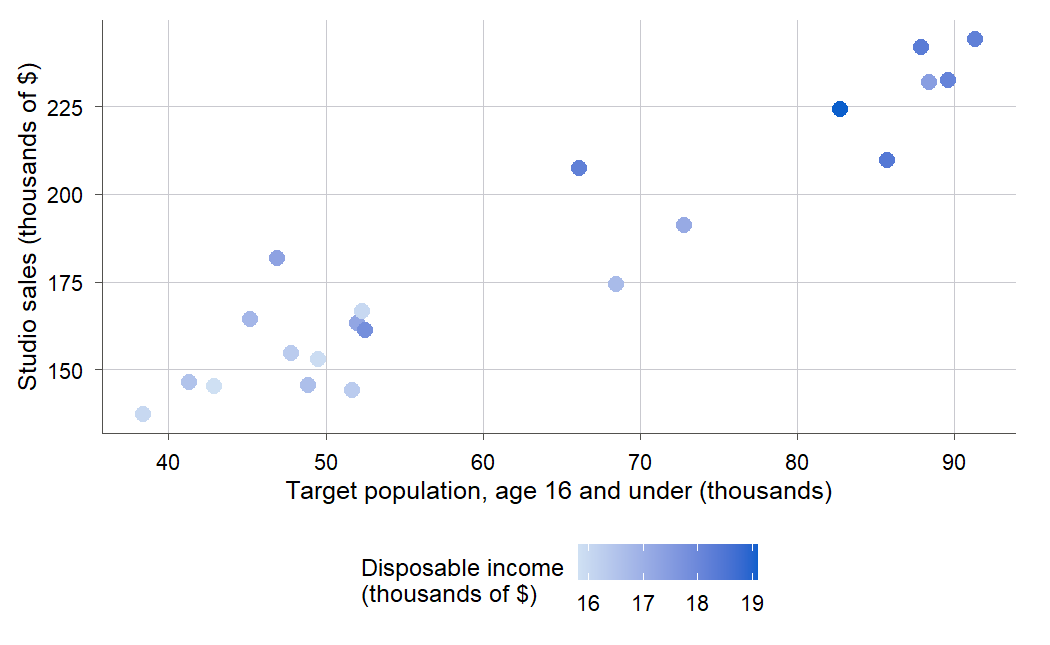
Figure 1:Dwaine Studios sales against a city’s under-16 population, with disposable income shown by shade. Both predictors track higher sales, so a good forecast needs to use them together, which is exactly what the matrix machinery in this chapter lets us do.
Figure 1 shows that both predictors matter: sales climb as the young population grows, and for a given population the higher-income cities (darker points) tend to sell more. A model that uses both at once is a multiple regression model, and every such model is built, fit, and understood through matrices. By the end you will have built, for the real Dwaine data, the design matrix , the product , its inverse, the coefficient estimates, the hat matrix, and every coefficient’s standard error, each from operations you can also do by hand on a small example.
6.1 The data as a vector and a matrix
Intuition
Start with the response. Dwaine has 21 sales figures, one per city. Stack them into a single column and you have a vector (Definition 6.1), an ordered list of numbers written vertically. Call it . A vector is the simplest matrix: many rows, one column.
Now the predictors. Each city carries two numbers, so the predictors form a table with 21 rows and 2 columns, and a table of numbers with rows and columns is a matrix (Definition 6.1). For regression we glue one extra column of all ones onto the front: a bookkeeping trick that lets the intercept ride along as just another coefficient. The result is the design matrix (Definition 6.2), with 21 rows and 3 columns. Figure 2 shows how the whole model lines up as stacked arrays.
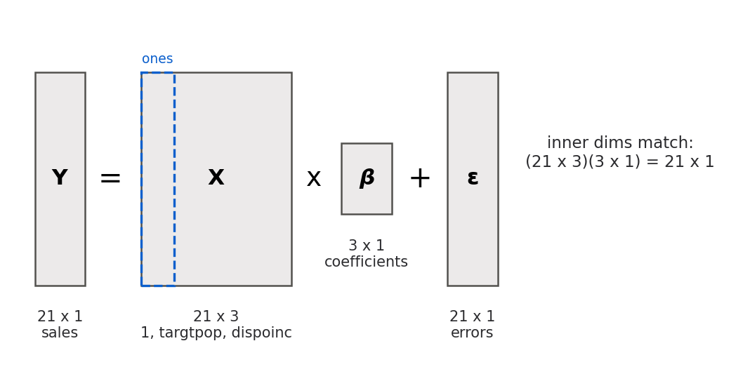
Figure 2:The regression model in matrix form. The response Y and errors are 21 by 1, the design matrix X is 21 by 3 with a leading column of ones for the intercept, and the coefficient vector beta is 3 by 1. The inner dimensions match, so the product is defined.
Reading across a row gives one city’s complete record: a 1, its young population, its disposable income, and, in , its sales. Stacking the rows turns 21 separate little equations into the single statement . That compression is the reason to learn matrices: the same three symbols describe a dataset with 21 rows or 21 million.
Formula
For a regression with observations and parameters (counting the intercept), the pieces are
is the response vector; row is the response for case .
is the design matrix; its first column is all ones, and column holds the values of predictor .
is the parameter vector: the intercept followed by the slopes.
is the number of regression parameters including the intercept ( for Dwaine), and is the number of observations ().
For Dwaine, and : one column of ones, one column of under-16 populations, one column of disposable incomes. The whole model of Chapter 2 generalizes to , which we unpack in 7.1 The model and least squares in matrix form. In words: each observed response equals a weighted sum of that row’s predictors, using the same weights for every row, plus a random error.
R and Python
6.2 Transpose and matrix multiplication
Intuition
We have the data in matrices; now we need to combine them. Two operations do almost all the work. The transpose (Definition 6.3) flips a matrix on its diagonal so rows become columns. Matrix multiplication (Definition 6.4) is the engine that turns the design matrix into the sums of squares and cross-products a regression runs on.
Matrix multiplication is not what a newcomer expects. One entry of the product is built from a whole row of the left matrix and a whole column of the right: line them up, multiply term by term, and add. Applied to , that rule produces exactly the sums you would otherwise compute one painful sum at a time. Figure 3 shows it on a small example.
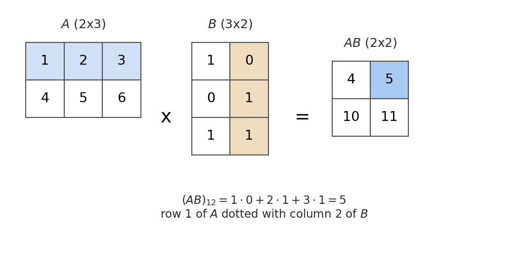
Figure 3:Matrix multiplication, entry by entry. The highlighted product entry in row 1, column 2 comes from row 1 of A and column 2 of B, multiplied term by term and summed. Every entry of a product is one such row-times-column dot product.
Two products, and only two, matter for the fit: summarizes the predictors by themselves, and summarizes how each predictor moves with the response. Between them they hold every summary least squares needs, which is why a whole dataset can shrink to a handful of numbers: the fit does not care about individual rows once these sums are known.
Formula
Picture it as tipping a matrix over its top-left corner: each row stands up to become a column, so a wide matrix tips into a tall one and back. A column vector, tipped over, becomes a single row, which is why multiplies a lying-down copy of a vector by a standing-up copy and collapses to one number.
The inner dimensions ( and ) must match; they are what you sum over.
The outer dimensions ( and ) give the shape of the answer.
Entry is row of dotted with column of .
Two products carry the whole load in regression. With of size , the transpose is , so
In words: collects every sum of squares and cross-product of the predictor columns into a small square table, and collects every predictor-times-response sum into a short column, the raw materials of the normal equations. A rule we will use constantly is that transposing a product reverses the order of its factors.
Proof. We show by comparing entries. The entry of is, by the definition of transpose, the entry of , which is . The entry of is row of dotted with column of , that is . The two sums have the same terms, so the matrices are equal.
R and Python
First the small example from Figure 3, so the mechanics are concrete
before we turn the engine loose on the real data. In R, %*% is matrix
multiplication (a plain * multiplies entry by entry instead); in Python the
operator is @.
A <- matrix(c(1, 2, 3,
              4, 5, 6), nrow = 2, byrow = TRUE)
B <- matrix(c(1, 0,
              0, 1,
              1, 1), nrow = 3, byrow = TRUE)
A %*% B
[,1] [,2]
[1,] 4 5
[2,] 10 11A = np.array([[1, 2, 3],
[4, 5, 6]])
B = np.array([[1, 0],
[0, 1],
[1, 1]])
print(A @ B)[[ 4 5]
[10 11]]The row-by-column rule is easier to trust once you have watched it happen on the one product a regression actually needs, so build yourself before moving on.
Tap or drag across any entry of the product and the row and column that made it light up, with the arithmetic spelled out underneath.
6.3 Identity, symmetry, independence, and rank
Intuition
Before inverting anything, we need vocabulary for the shapes of matrices that show up in regression, and one idea that decides whether a fit is even possible. The identity matrix (Definition 6.6) is the matrix version of the number 1: multiplying by it changes nothing. A symmetric matrix (Definition 6.7) equals its own transpose, and is always symmetric, which is why its table looks like a mirror across the diagonal.
The idea that decides feasibility is linear independence (Definition 6.8) of
the predictor columns. If one predictor column is an exact linear combination of
the others, say dispoinc were exactly twice targtpop plus a constant, then the
columns carry redundant information, the matrix is rank deficient,
and
cannot be inverted. There is then no unique best fit,
because the data cannot tell the redundant coefficients apart. This is the matrix
face of a problem you will meet again as multicollinearity in 12.1 Multicollinearity and the variance inflation factor.
A picture makes independence concrete. Think of two columns as arrows drawn from the origin. If they point in genuinely different directions, they open up an area between them, and the matrix has full rank. If one is just a stretched copy of the other, both arrows lie on a single line, the area between them is zero, and the matrix is rank deficient. Figure 5 shows both cases side by side.
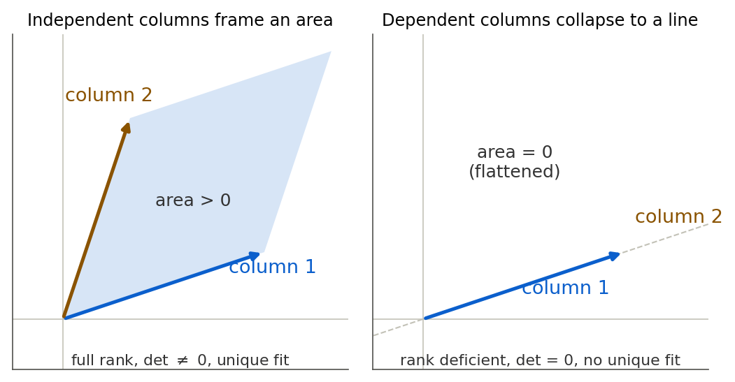
Figure 5:Rank seen as geometry. Independent columns spread out and enclose an area, so the fit is unique; dependent columns fall on one line and enclose nothing, so the fit is not. The enclosed area is exactly the determinant of the next section, and its collapse to zero is what makes a matrix singular.
These names earn their keep: a named property is a fact you can cite instead of recompute. Showing the hat matrix is a projection becomes a one-line argument, “it is symmetric and idempotent,” in place of pages of entry-by-entry checking.
Formula
The product is always symmetric, because by the order-reversing rule (Theorem 6.5) of 6.2 Transpose and matrix multiplication.
The central fact of this section connects rank to invertibility.
A tiny example makes rank concrete: and are independent, but and are dependent because the second is exactly twice the first, so together they span only a line and have rank 1, not 2. In a design matrix, such a dependent column is a predictor that repeats information already present.
R and Python
Software reports symmetry, rank, and the determinant (the single number, covered in 6.4 The inverse and the normal equations, whose vanishing signals rank deficiency) directly.
isSymmetric(XtX)
qr(X)$rank
round(det(XtX), 2)
[1] TRUE
[1] 3
[1] 1068302print(np.allclose(XtX, XtX.T))
print(np.linalg.matrix_rank(X))
print(round(np.linalg.det(XtX), 2))True
3
1068302.4The design matrix has rank 3, its full column count, so the two predictors plus the intercept carry three genuinely different pieces of information, and the nonzero determinant confirms that is invertible and the Dwaine fit is well posed.
The habit to build: before trusting any multiple regression, ask whether the predictors are genuinely distinct. Software will happily invert a nearly singular matrix and return coefficients with enormous standard errors, the early warning that two predictors carry almost the same information. Rank is the yes-or-no version of that question; Chapter 12 sharpens it into “how close to dependent are they?”
6.4 The inverse and the normal equations
Intuition
Here is where the machinery pays off. In ordinary algebra, to solve you divide by , which is the same as multiplying by . Matrices have no division, but they have the next best thing: for a square matrix with full rank, there is an inverse (Definition 6.10) that undoes it, meaning . To solve a matrix equation , multiply both sides on the left by and get .
The normal equations of least squares, which in Chapter 2 were two scalar equations, collapse in matrix form to the single equation . Chapter 7 derives this from minimizing squared error (7.1 The model and least squares in matrix form); for now take it as the matrix twin of the Chapter 2 normal equations (2.2 Least squares from first principles). Solving it is now a one-liner: multiply by .
With numbers, exists for every except zero. With matrices, exists for every square matrix except the rank-deficient ones, so “can I solve this uniquely,” “is the determinant nonzero,” and “are the columns independent” are three ways of asking one question. For Dwaine, all three say yes.
Formula
The determinant measures whether the columns are independent; if it is zero, the inverse formula divides by zero and no inverse exists.
For larger matrices the determinant is more involved, so we let software compute it, but the rule “invertible if and only if determinant nonzero” stays exact.
This connects back to the picture of rank in Figure 5: the two columns of a two-by-two matrix frame a parallelogram, and the determinant is its area. When the columns point along the same line the parallelogram is squashed flat, its area is zero, and the matrix is singular, so “determinant zero” and “the columns collapse onto one line” are the same event.
Applying the inverse to the normal equations gives the least-squares estimator in one line.
In words: multiply the stored cross-products by the inverse of the cross-product matrix , and out come all coefficient estimates at once. This one formula is the whole of least-squares estimation, for any number of predictors.
R and Python
First the inverse formula, checked on a small symmetric matrix, so
you can see happen. Both languages invert
with a single call: solve in R, np.linalg.inv in Python.
M <- matrix(c(2, 1,
              1, 2), nrow = 2, byrow = TRUE)
Minv <- solve(M)
Minv
round(M %*% Minv, 6)
[,1] [,2]
[1,] 0.6666667 -0.3333333
[2,] -0.3333333 0.6666667
[,1] [,2]
[1,] 1 0
[2,] 0 1M = np.array([[2.0, 1.0],
[1.0, 2.0]])
Minv = np.linalg.inv(M)
print(Minv)
print(np.round(M @ Minv, 6))[[ 0.66666667 -0.33333333]
[-0.33333333 0.66666667]]
[[1. 0.]
[0. 1.]]The determinant is , so the inverse is , matching the printout, and returns the identity.
You will almost never invert a matrix bigger than this by hand; working the
two-by-two case once is enough to see where the answer comes from and watch the
identity appear, so a software inverse is never magic. From here on we let solve
and np.linalg.inv do the arithmetic, and the next example turns the inverse loose
on the full Dwaine fit.
A determinant of zero is easier to feel than to define, so pull the two columns together yourself and watch the inverse come apart long before they meet.
Drag either column arrow. The shaded box has area equal to the size of the determinant, and the entries of the inverse grow without bound as that box flattens.
6.5 Idempotent and projection matrices
Intuition
The coefficients are done, so the model can now make its own predictions. The question of this section is where those predictions come from and what they look like as a picture. The answer is a single table of numbers that turns the observed sales into the model’s fitted sales in one step, and that step is a shadow: it flattens the data onto the surface the predictors can reach.
With in hand, the fitted values are . Substitute the estimator and something remarkable appears:
Geometrically the hat matrix is a projection (Definition 6.14). Picture as an arrow in -dimensional space; the fitted values a regression can produce all lie in a flat subspace, the span of the columns of . The hat matrix drops straight down onto that subspace, landing at the closest point, and the residual is the perpendicular leftover. Figure 7 shows this picture, the subject of 7.2 The geometry of least squares.
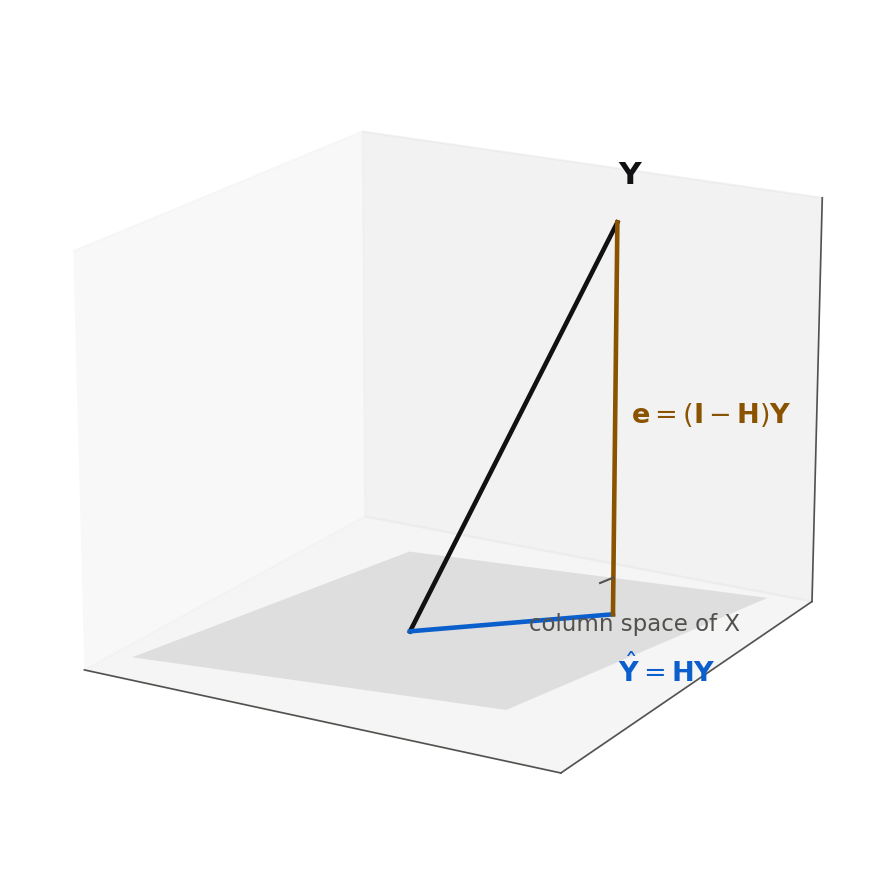
Figure 7:Least squares as a projection. The fitted vector Y-hat is the shadow of the response Y on the column space of X, and the residual e joins them at a right angle. The hat matrix H performs the projection onto the plane; I minus H produces the perpendicular residual.
Two algebraic properties make a projection, and they are the workhorses of the diagnostics in Chapter 9. First, is symmetric. Second, is idempotent: applying it twice is the same as applying it once, . That makes sense for a projection, since once a vector is flattened onto the plane, flattening again does nothing.
The shadow picture is worth holding onto. Your shadow on flat ground keeps your left-right and forward-back position but flattens your height to zero; the hat matrix does the same to , flattening away the part of the response that no combination of the predictors could reproduce, which is the residual.
These properties are not decoration: Chapter 9 reads the diagonal of to find which cities pull hardest on the fitted surface, Chapter 7 uses its trace to count degrees of freedom, and the perpendicular picture is what makes least squares the closest fit, with no point in the plane nearer to than its own shadow.
Formula
The two projections of regression are
with the fitted values and the residuals. In words: projects onto the space of fittable values, and projects onto the leftover space of residuals.
The two defining properties of are what make it a projection.
Proof. Write , which is symmetric because is (its inverse inherits symmetry: ). For symmetry of , apply the order-reversing transpose rule of 6.2 Transpose and matrix multiplication twice:
For idempotency, multiply by itself and cancel the inner against its inverse:
using . The same two steps show is symmetric and idempotent: .
R and Python
The projection is the one idea in this chapter a flat page cannot really show, so turn the picture around and move with your own finger.
Drag the tip of Y anywhere in space. Yhat stays on the column space of X and the residual e stays perpendicular to it, which is exactly what makes the fit the closest one available.
6.6 Quadratic forms and sums of squares
Intuition
Every “sum of squares” in regression is secretly one matrix expression called a quadratic form (Definition 6.17). The error sum of squares is , and a sum of squared entries of a vector is exactly that vector dotted with itself: . Because , a little algebra rewrites SSE using only and a projection matrix in the middle. That middle-matrix pattern, , is a quadratic form, and SSTO, SSR, and SSE are all of this shape.
Why care? Two reasons. First, a quadratic form makes the degrees of freedom and the expected value of each sum of squares fall out of the middle matrix, how Chapter 7 explains the ANOVA table. Second, sums of squares can never be negative, and that is guaranteed by a property of the middle matrix called positive semidefiniteness. Figure 9 shows why a positive-definite form is shaped like a bowl that never dips below zero.
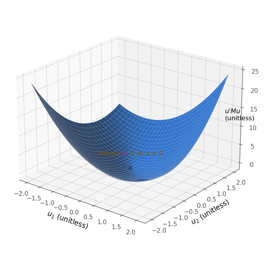
Figure 9:A positive-definite quadratic form is a bowl. Its value is zero only at the origin and strictly positive in every other direction, which is exactly why a sum of squares written as such a form can never be negative.
The payoff is that this view survives even when the sum no longer looks like a sum of squares. Written as , SSE does not visibly square anything, yet the middle matrix still guarantees it cannot go negative. The same reasoning applies to a variance, a sum of squares in disguise, so the covariance matrix of the next section can never hold a negative variance.
Formula
The three regression sums of squares are all quadratic forms in , and their middle matrices carry the ANOVA decomposition.
Proof (nonnegativity). Because is symmetric and idempotent, , so SSE is a genuine sum of squares and can never be negative; the same holds for SSR and SSTO. The additive decomposition of the middle matrices is the matrix statement of the ANOVA identity (3.6 The analysis of variance approach).
In words: the sums of squares are quadratic forms, and the idempotent middle matrices both guarantee nonnegativity and, in Chapter 7, hand us the degrees of freedom through their traces.
R and Python
6.7 Random vectors, expectation, and covariance matrices
Intuition
So far the matrices held fixed numbers. But is random: rerun the 21 cities under the same conditions and the sales would come out a little different, because of the errors . To describe a vector of random variables we need two things: a vector of means and a table of variances and covariances.
The vector of means is just the expectation applied entry by entry. The table is the covariance matrix (Definition 6.19): its diagonal holds the variance of each entry, and its off-diagonals hold the covariance between pairs of entries. For the regression errors, this table is simple: constant variance down the diagonal (every error has the same spread) and zeros off it (distinct errors are uncorrelated), so . A two-line rule for how means and covariances travel through a linear map then yields the covariance matrix of , the source of every standard error.
Formula
The transformation rules for how these travel through a linear map are the heart of the section.
In words: expectation passes straight through a linear map, and a covariance matrix gets sandwiched between and its transpose. Apply these to the regression model, where and , and the mean and covariance of follow.
Proof. The estimator is a linear map of : with , we have . For the mean, use :
so is unbiased for . For the covariance, use and the sandwich rule:
where the middle cancels one inverse. So : the same inverse we used to compute also gives, once scaled by , the variance of every coefficient and the covariance of every pair.
Replacing the unknown by its estimate MSE gives the estimated covariance matrix , whose diagonal square roots are the standard errors that software prints.
R and Python
6.8 The multivariate normal, in brief
Intuition
The mean vector and covariance matrix describe a random vector’s center and spread, but not its full shape. For inference we add one assumption, the same one that turned Chapter 2’s estimates into tests: the errors are normal. Stacked into a vector, normal errors with constant variance and no correlation follow a multivariate normal distribution (Definition 6.22), the several-variable generalization of the bell curve. Its contours are ellipses whose tilt and stretch are read directly off the covariance matrix, as in Figure 10.
What the full distribution adds is how the probability thins out as you move from the center: the same bell-curve falloff you know from one variable, measured along the tilted axes of the covariance ellipse. That is what lets us compute the chance that a coefficient lands within a stated distance of the truth, exactly what a confidence interval reports in the next chapter.
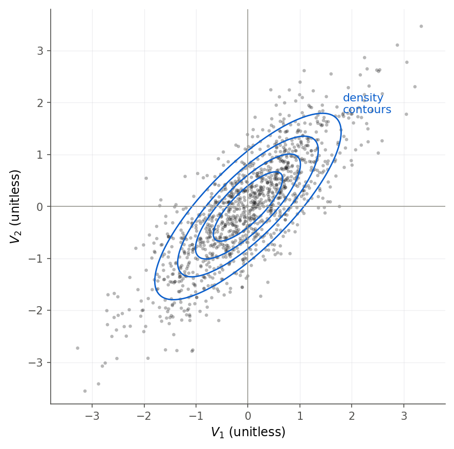
Figure 10:A bivariate normal distribution. The two coordinates have covariance 0.8, so the cloud and its elliptical contours tilt along the diagonal. The shape of the ellipse is exactly the covariance matrix, which is why the sampling distribution of the coefficient vector b is described by its covariance matrix.
Why this matters: under normal errors the response is multivariate normal, and because is a linear map of , so is . That fact, , is the foundation of every confidence interval, test, and test ahead.
One caution keeps this honest. Multivariate normality of is a consequence of assuming normal errors, not a fact the data hand you for free. If the errors are badly non-normal and the sample is small, that law is only approximate, one reason Chapter 5’s permutation and bootstrap methods exist (5.4 The bootstrap for regression). With a large sample, an averaging effect pulls toward normal even when the errors are not.
Formula
Applying that property to regression under the normal error model gives the sampling law that drives every later inference.
The response is centered at the regression surface with independent, equal-variance coordinates, and the estimator is centered at the truth (unbiased) with the covariance matrix we derived.
In words: normal errors make both the data and the estimates normal, so every coefficient is normally distributed with a variance we can read from , and that is what makes exact inference possible.
R and Python
We can demonstrate the covariance-recovery idea by simulation: draw many vectors with a target covariance and confirm the sample covariance matches. Starting from independent standard normals , the transformation , where is a matrix square root of the target (the Cholesky factor), produces vectors with covariance , exactly the sandwich rule at work.
set.seed(4210)
mu <- c(0, 0)
Sigma <- matrix(c(1, 0.8,
                  0.8, 1), nrow = 2)
L <- chol(Sigma)
Z <- matrix(rnorm(2 * 5000), ncol = 2)
V <- Z %*% L
round(cov(V), 3)
[,1] [,2]
[1,] 0.967 0.760
[2,] 0.760 0.955rng = np.random.default_rng(4210)
Sigma = np.array([[1.0, 0.8],
[0.8, 1.0]])
L = np.linalg.cholesky(Sigma)
Z = rng.standard_normal((5000, 2))
V = Z @ L.T
print(np.round(np.cov(V, rowvar=False), 3))[[1.017 0.822]
[0.822 1.026]]The sample covariance of the 5000 simulated vectors comes out close to the target in both languages, differing only by sampling noise.
The Cholesky factor can stay a black box for now; the point is that a covariance can be planted on purpose, by passing uncorrelated noise through a fixed matrix and letting the sandwich rule do the rest. The covariance of is the same story: error noise passed through the fixed matrix , so the simulation and the regression are two uses of one mechanism.
6.9 Chapter summary
You can now speak the matrix language the rest of the book is written in: lay a dataset out as a response vector and a design matrix , build the products and every fit runs on, tell when a matrix is invertible, solve the normal equations for , build the hat matrix and prove it is a projection, express the sums of squares as quadratic forms, and find the mean and covariance of a random vector. For the real Dwaine data, all of this was computed in both R and numpy: , on 18 degrees of freedom, , and standard errors . From these tools came the two facts that drive all of multiple regression: is unbiased, and its covariance is .
Every piece fits into one pipeline, drawn in Figure 11: from the data you form two summaries, invert one of them, and everything else, the coefficients, the hat matrix, the residuals, and the standard errors, drops out in a fixed order. If you remember the shape of that pipeline, you can rebuild any single formula in it.
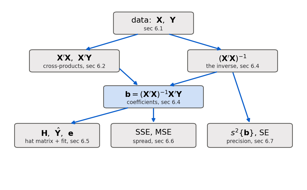
Figure 11:The chapter as one pipeline. Every quantity of a multiple regression fit, the coefficients, fitted values, residuals, error variance, and standard errors, comes from the same two cross-product summaries and a single inverse, computed in a fixed order.
Key results at a glance.
| Result | Statement or formula | Valid when |
|---|---|---|
| Transpose of a product (Theorem 6.5) | any conformable | |
| Invertibility criterion (Theorem 6.9) | invertible has full column rank | square |
| Least-squares solution (Theorem 6.12) | full column rank | |
| Hat matrix is a projection (Theorem 6.16) | symmetric, idempotent, | full column rank |
| Sums of squares as quadratic forms (Theorem 6.18) | ; ; | any response |
| Linear transformation rules (Theorem 6.20) | ; | fixed |
| Mean and covariance of (Theorem 6.21) | ; | , |
| Sampling distribution of (Theorem 6.23) | normal errors |
Key terms. matrix, vector, design matrix, transpose, matrix multiplication, conformable, identity matrix, symmetric matrix, linear independence, rank, determinant, inverse, normal equations, hat matrix, idempotent matrix, projection matrix, trace, quadratic form, positive definite, random vector, covariance matrix, multivariate normal.
You should now be able to.
Represent a regression dataset as a response vector and a design matrix , and write the model as .
Compute transposes and matrix products, and build and by hand and with software.
Decide when a square matrix has an inverse using rank and the determinant, and explain what perfect collinearity does to .
Solve the normal equations for .
Verify that the hat matrix is symmetric and idempotent, and explain why fitted values and residuals are projections.
Express SSE, SSR, and SSTO as quadratic forms, and connect positive definiteness to nonnegative sums of squares.
Derive the mean vector and covariance matrix of a random vector, and use them to show .
State the multivariate normal model for and and describe how it powers the inference of later chapters.
Where this fits. This chapter is the toolbox that makes the FIT and USE stages of the course workflow (The modeling workflow) work for more than one predictor: the estimator fits every multiple regression, and the covariance matrix is how every coefficient is later tested. Chapter 2 built these ideas for one predictor with scalar algebra (2.2 Least squares from first principles); we have now generalized them to any number. Next, Chapter 7 takes the same Dwaine you computed and proves why these formulas are the right ones: it derives least squares two ways (7.1 The model and least squares in matrix form), reads the degrees of freedom off the hat matrix (7.3 The hat matrix), and proves the Gauss-Markov theorem (7.6 The Gauss-Markov theorem). It is the most abstract chapter in the course, and it is built almost entirely from the matrix facts you assembled here, so the work of this chapter is exactly what makes the next one readable.
6.10 Frequently asked questions
Q1. Why do we glue a column of ones onto ? So the intercept can be treated as just another coefficient. Multiplying the ones column by gives in every row, which is exactly what an intercept does. Without the ones column, the formula would have no constant term, and you would be forcing the regression surface through the origin.
Q2. Is the same as squaring ? No. is usually not square, so is not even defined. multiplies the transpose () by () to make a matrix of sums of products. It is the closest matrix analogue of “sum of squares,” which is why it sits at the center of least squares.
Q3. What actually goes wrong when is singular? Two predictor columns carry the same information, so the data cannot decide how to split an effect between them. Infinitely many coefficient vectors fit equally well, the inverse does not exist, and software either errors out or silently drops a predictor. This is the extreme end of the multicollinearity you meet in 12.1 Multicollinearity and the variance inflation factor.
Q4. Do I have to invert by hand? No. Past ,
let solve or np.linalg.inv do it, and in real work prefer the routines inside
lm and statsmodels, which solve the normal equations without forming the
inverse. Computing the inverse here just shows that the software does exactly the
matrix algebra of this chapter, so it is never a black box.
Q5. Why is the hat matrix called a projection? Because it takes the response vector and drops it perpendicularly onto the flat subspace of all fittable values (the column space of ), landing at the closest point, . Projecting a second time changes nothing, which is the algebraic property . The residual is the part of left sticking out, at a right angle to the subspace.
Q6. Where does the normal distribution enter? Only in 6.8 The multivariate normal, in brief, and only for inference. Building , computing , the hat matrix, SSE, and the covariance matrix all use no distributional assumption beyond mean zero, constant variance, and uncorrelated errors. Normality is added on top so that is multivariate normal and we can build exact and procedures, which is Chapter 7’s job.
Q7. Do I have to memorize all these identities, and should the negative entries in the covariance matrix of worry me? No on both counts. Hold on to three things: the model , the estimator , and the covariance ; everything else builds one of those or reads a number out of it, so the identities become things you rederive rather than recall. As for the negative entries, only the off-diagonal covariances can go negative (the diagonal variances never do), and a negative one between two slopes just means that across repeated samples overestimating one tends to accompany underestimating the other. It is information, not an error.
6.11 Practice problems
(A) Give the dimensions of , , , , , and for the Dwaine model, and say in one phrase what each represents.
(A) Explain why the first column of the design matrix is all ones, and what would change in the model if it were removed.
(A) State the rule for when two matrices can be multiplied, and use it to explain why is undefined for the Dwaine design matrix but is defined.
(A) In words, what is the entry in row 1, column 1 of equal to, and why? What are the other entries of the first row?
(A) Define an idempotent matrix and a symmetric matrix, and state which of these properties the hat matrix has.
(A) A colleague writes and “cancels ” from . Explain the two things wrong with this.
(A) Explain what it means for the columns of to be linearly dependent, and what that does to and to the least-squares fit.
(A) The covariance matrix of has a negative off-diagonal entry between the two slopes. Interpret its sign in one sentence.
(B) Prove that is symmetric for any matrix , citing the transpose-of-a-product rule (Theorem 6.5).
(B) Prove the transpose-of-a-product rule (Theorem 6.5), , by comparing the entries of both sides.
(B) Starting from the matrix normal equations , derive (Theorem 6.12), stating the condition on that the step requires.
(B) Prove that the hat matrix is symmetric and idempotent (Theorem 6.16). Then show is idempotent.
(B) Show that , and explain geometrically why projecting each column of onto the column space of leaves it unchanged.
(B) Using and , prove that and that (fitted values are orthogonal to residuals).
(B) Prove the covariance transformation rule (part of Theorem 6.20) for a fixed matrix , starting from the definition .
(B) Use the rules of problem 15 and , to derive and (Theorem 6.21).
(B) Show that equals (Theorem 6.18), using the symmetry and idempotency of , and explain why this proves .
(B) For the matrix , write the quadratic form in terms of , and give a condition on that makes it positive definite.
(B) The fitted values satisfy . Prove that and , using the covariance rule and the properties of .
(C) Read
dwaine.csv, build and , and reproduce and in R or Python. Confirm the top-left entry of is and the first entry of is .(C) Compute and in software, and check that matches
lm/statsmodelsand that returns the identity.(C) Build the hat matrix , verify numerically that and that , and report the three largest diagonal entries (the leverage values).
(C) Compute the residual vector and verify numerically that (all three entries near zero) and that .
(C) Compute , then and , and confirm they match the residual standard error reported by
summary(fit)/fit.summary().(C) Form the estimated covariance matrix and report the three standard errors from its diagonal. Confirm they match the software summary, and report the estimated covariance between the two slope estimates.
(C) Predict sales for a new city with and by forming the row vector and computing . Confirm the result against
predict.(C) Add a redundant column to equal to , and try to compute . Report what R or Python does (an error, a warning, or a wildly unstable inverse), and connect it to rank deficiency.
(C) Center the predictors: replace
targtpopanddispoincby their deviations from their means, refit, and confirm that the two slopes are unchanged while the intercept becomes . Explain, using the normal equations, why centering leaves the slopes alone.(C) Demonstrate the sampling law (Theorem 6.23, 6.8 The multivariate normal, in brief) by simulation. Treat the fitted as the true and as the true . Holding the real Dwaine fixed, use
set.seed(4210)(R) ordefault_rng(4210)(Python) to generate 5000 response vectors with , refit each by , and collect the estimates. (a) Confirm the column means are close to and the sample covariance is close to . (b) In two sentences, explain why this law lets Chapter 7 attach a distribution to each coefficient and turn a standard error into a confidence interval.
6.12 Exam practice
These five questions match the style of the course exams: each asks you to
explain, evaluate, or interpret in full sentences, not to produce a bare number.
Write in complete sentences and say which numbers you used. The software output
shown was generated from the real dwaine.csv fit. Each model answer shows the
depth that earns full marks, followed by one line on what a weak answer misses.
EP 6.1. In the Dwaine fit both estimated slopes are positive: and . A student argues, “since both predictors push sales up, the two slope estimates must be positively correlated across repeated samples.” The estimated covariance matrix of is printed below. Evaluate the student’s claim, and explain what the relevant number actually tells you.
          intercept targtpop  dispoinc
intercept 3602.0347   8.7459 -241.4230
targtpop     8.7459    0.0449   -0.6724
dispoinc  -241.4230   -0.6724   16.5158
Model answer
The claim confuses the sign of the coefficients with the sign of the covariance between their estimators, and the two are unrelated. The number that settles the question is the off-diagonal entry between the two slopes, , which is negative. So across repeated samples an overestimate of one slope tends to arrive with an underestimate of the other, exactly the opposite of what the student predicts. That negative sign comes from the geometry of the design matrix: the two predictor columns are themselves positively correlated across the 21 cities, so the fit cannot raise both slopes at once without double-counting the shared signal, and it trades one off against the other. The signs of the fitted slopes, which describe how sales respond to each predictor, carry no information about how the two estimates co-vary. A weak answer just declares the claim true or false, or repeats that both slopes are positive, without reading the -0.6724 entry and explaining that it is negative for reasons tied to the predictors, not the coefficients.
EP 6.2. Suppose targtpop is re-entered in raw persons instead of thousands,
so every value is multiplied by 1000, and the model is refit. Using the output
below, state precisely which quantities change and which stay identical, and
explain why.
          b            se           t
intercept -68.8570732  60.0169532  -1.1473
targtpop    0.0014546   0.0002118   6.8682
dispoinc    9.3655004   4.0639581   2.3045
SSE = 2180.9274      fitted[1:3] = 187.184, 154.229, 234.396
Model answer
Multiplying one predictor column by 1000 divides that predictor’s slope and the
slope’s standard error by the same factor of 1000: the targtpop slope falls
from 1.4546 to 0.0014546 and its standard error from 0.2118 to 0.0002118,
so their ratio, the statistic 6.868, is unchanged. Everything else is
identical to the original fit: the intercept -68.857, the dispoinc slope
9.3655, all fitted values (187.184, 154.229, 234.396, ...), the residuals,
, , and . The reason is that scaling a
column of by a nonzero constant does not change the column space that
spans, and the fit depends on only through that space:
the hat matrix , the projection ,
and every sum of squares are untouched. A change of units therefore rescales the
affected coefficient and its standard error in lockstep and leaves every fitted
value and every inference alone. A weak answer says only that “the slope changes”
without noting that its standard error changes by the identical factor, that the
statistic, fitted values, and SSE are invariant, and why.
EP 6.3. The diagonal of the hat matrix holds the leverage values . The output below reports their sum, the rule-of-thumb cutoff, and the five largest values with the two predictor values of each city. Interpret these numbers in context: what do they say about which cities matter most, why do they sum to 3, and would you flag any city as a high-leverage point?
sum of h_ii = 3.0        2p/n cutoff = 0.2857
 city 20:  targtpop 82.7  dispoinc 19.1   h = 0.2788
 city 13:  targtpop 88.4  dispoinc 17.4   h = 0.2390
 city 15:  targtpop 52.5  dispoinc 17.8   h = 0.2095
 city  3:  targtpop 91.3  dispoinc 18.2   h = 0.1737
 city  5:  targtpop 46.9  dispoinc 17.3   h = 0.1620
Model answer
Each leverage value measures how far city ’s predictor values sit from the center of the predictor cloud, and it equals the weight that the city’s own sales carry in producing its fitted value. City 20 has the largest leverage value () because it pairs a large young population (82.7 thousand) with the highest disposable income in the data (19.1), so it sits at the outer edge of the predictor cloud and its response has the biggest say in the local fit. The leverages sum to 3 because , the number of estimated parameters, so on average a city carries of its own fitted value; this is the same trace fact that produces the divisor for . Comparing against the cutoff, no city exceeds it, since even city 20 at 0.2788 falls just under, so none is flagged as an unusually high-leverage point, though city 20 is the one to watch. A weak answer reads off the largest number without saying what a leverage value measures, misses that the sum equals because , or calls a city high-leverage from its raw size without comparing to the 0.2857 cutoff.
EP 6.4. A student augments the Dwaine design matrix with a fourth column equal
to targtpop + dispoinc, refits, and reports: “Python still returned an inverse
and some coefficients, so the augmented model is fine.” The diagnostics below come
from the augmented matrix. Explain why the augmented model is not fine, what has
gone wrong mathematically, and why R and Python behave differently.
rank of augmented X = 3   (it has 4 columns)
det(X'X)        = -3.7e-05      # against ~1.07e06 for the genuine 3x3 X'X
R  solve(X'X):  Error: system is computationally singular
Python inv(X'X): returns a matrix of enormous (~1e13) entries, no error
Model answer
The new column is an exact linear combination of two existing columns, namely
, so the four columns are linearly dependent and
the design matrix has rank 3, not 4. By Theorem 6.9, is
then singular and has no genuine inverse: its true determinant is zero, and the
printed is floating-point dust around zero, astronomically
small next to the roughly determinant of the real
. There is no unique least-squares solution, because the data
cannot decide how to split an effect between a predictor and a copy built from it;
infinitely many coefficient vectors fit equally well. R computes the reciprocal
condition number, sees it is essentially zero, and refuses with “system is
computationally singular,” which is the honest response. Python’s np.linalg.inv
inverts without checking conditioning, so it returns a matrix of enormous,
meaningless entries that are numerical noise rather than a fit. The student has
mistaken a silent numerical failure for a valid model: the fact that code “ran” is
no evidence the answer means anything. A weak answer notes only that the columns
are collinear without connecting rank deficiency to the zero determinant and the
absence of a unique solution, or trusts Python’s numbers because no error appeared.
EP 6.5. A regional manager wants the model’s predicted mean sales for a new
city with targtpop and dispoinc , together with a standard
error, so form and note that the predicted mean
is . The estimated covariance matrix
is reprinted below,
and the fit gives . A student computes the standard error
of as ,
using only the diagonal variances. Explain why this is wrong, give the correct
standard error, and say which way the diagonal-only shortcut errs.
          intercept targtpop  dispoinc
intercept 3602.0347   8.7459 -241.4230
targtpop     8.7459    0.0449   -0.6724
dispoinc  -241.4230   -0.6724   16.5158

x_h'(X'X)^{-1} x_h = 0.063181       MSE = 121.16
Model answer
The predicted mean is a linear
combination of all three coefficients, so by the covariance rule of Theorem 6.20
its variance is the full quadratic form
,
which includes every off-diagonal covariance, not only the three diagonal
variances. The student’s shortcut drops the cross terms
, and here those terms are large and negative,
above all the -241.42 covariance between the intercept and the dispoinc slope,
so ignoring them wildly overstates the variance. Computing it correctly,
,
so the standard error is thousand dollars, not 94.4. The
diagonal-only shortcut errs by a huge margin on the high side, because the negative
covariances that the coefficients genuinely have would cancel much of the diagonal
contribution. The lesson is that the standard error of any linear combination of
needs the whole covariance matrix, since the coefficients are
correlated. A weak answer computes
as a formula without explaining that the missing off-diagonal terms are what make
the shortcut wrong, or fails to note that the shortcut overstates rather than
understates the standard error.
6.13 Chapter game
Resumen del capítulo (en español)
Este capítulo enseña el álgebra de matrices (matrix algebra) que necesita la regresión múltiple, sin suponer conocimientos previos de álgebra lineal. Usa los datos de Dwaine Studios: las ventas de 21 estudios de retratos frente a dos predictores, la población menor de 16 años y el ingreso disponible per cápita. Los datos se organizan en un vector respuesta (response vector) y una matriz de diseño (design matrix) de tamaño , cuya primera columna es de unos para el intercepto, y el modelo se escribe de forma compacta como .
Definimos la transpuesta (transpose) y la multiplicación de matrices
(matrix multiplication), cuya regla es “fila por columna”, y con ellas
construimos las dos piezas centrales: , que reúne todas las
sumas de cuadrados y productos cruzados, y . Una matriz
tiene inversa (inverse) solo si tiene rango completo, equivalentemente si su
determinante (determinant) no es cero. Al resolver las ecuaciones normales
se obtiene el estimador
; para Dwaine,
, idéntico al de lm y statsmodels.
La matriz sombrero (hat matrix) es simétrica e idempotente (idempotent): proyecta sobre los valores ajustados. Las sumas de cuadrados SSE, SSR y SSTO son formas cuadráticas (quadratic forms), y para Dwaine con sobre 18 grados de libertad. Para un vector aleatorio (random vector), la esperanza y la matriz de covarianzas se transforman según y , de donde es insesgado y . Bajo errores normales, sigue una distribución normal multivariante (multivariate normal), base de toda la inferencia del Capítulo 7.