We return to the Dwaine Studios cities of Chapters 6 and 7 (7.1 The model and least squares in matrix form), where a chain of
portrait studios in mid-sized towns wants to decide, for a city it has never entered, how much a new
studio will sell. Two recorded numbers about each of its 21 cities plausibly drive that answer: the
target population targtpop (thousands of persons under 16, the pool of potential family-portrait
customers) and the disposable income dispoinc (thousands of dollars per person, how much those
families have to spend), together predicting annual sales (thousands of dollars).
In Chapter 6 we built this data into matrices, and in Chapter 7 we solved the normal equations to get the least-squares coefficients ; see 7.1 The model and least squares in matrix form. That was the FIT stage. This chapter is about what comes after: reading those three numbers honestly, deciding which predictors are earning their place, and knowing the traps that wait for anyone who reports a coefficient without thinking. Figure 1 shows the raw material, sales against each predictor one at a time.
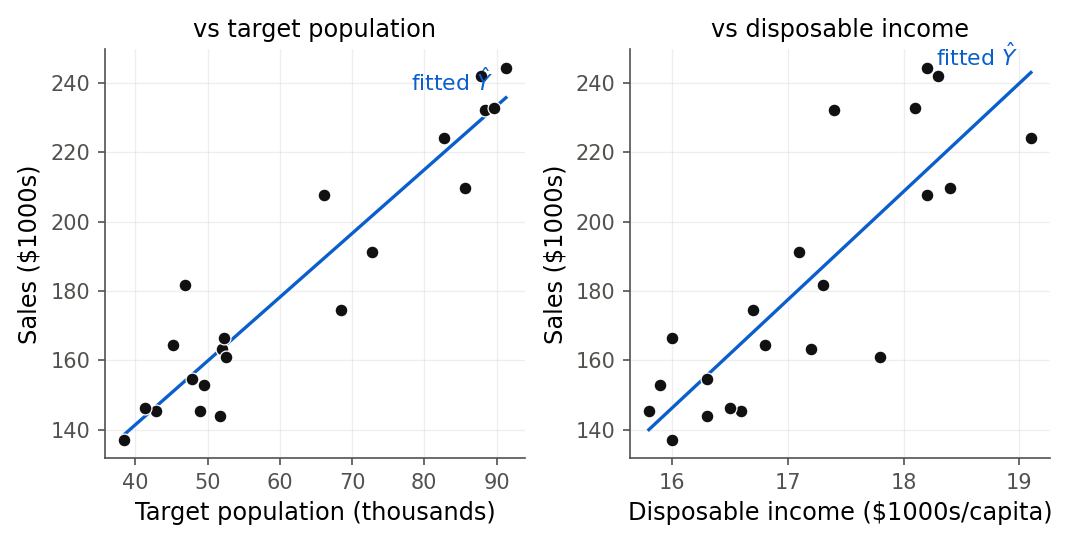
Figure 1:Dwaine sales against each predictor separately. Both slopes are positive: bigger target population and higher income each go with higher sales. The chapter’s work is to untangle these two overlapping stories into one model that holds both at once.
Both pictures slope up, so both predictors look useful. But the two predictors also move together (richer cities tend to have different age profiles), and that overlap is the whole difficulty of multiple regression. A coefficient in a multiple regression is not the slope you would see in a one-predictor scatterplot. It answers a more careful question, and this chapter is about asking that question correctly, testing whether a predictor belongs, and seeing the answer in a picture.
8.1 Reading the coefficients of a multiple regression
Intuition
The fit handed us three numbers. This section is about what each one honestly means, because the obvious reading is the wrong one. The short version: a number in a multiple regression answers a more careful question than the same-looking number in a one-predictor plot.
The Dwaine fit is . It is tempting to read the 9.37 the same way we read a simple-regression slope: “raise income by one unit and sales go up 9.37.” That reading is wrong in a specific and important way. In a one-predictor world, moving income means moving whatever else travels with income. In the multiple regression, the coefficient on income has already accounted for target population. It measures what income adds after target population has said everything it can say.
The clean phrase is: a multiple regression coefficient is a partial slope (Definition 8.1). It is the change in the mean response for a one-unit change in that predictor, holding the other predictors fixed. “Holding fixed” is what makes it different from the marginal picture in Figure 1, where nothing is held fixed and every predictor drifts along with every other.
Formula
The multiple linear regression model with predictors is stated in Definition 8.2.
Term by term:
is the response for case (Dwaine sales for city ).
is the -th predictor for case .
is the partial slope for predictor : the change in per one-unit rise in with every other predictor held fixed.
is the intercept, the mean response when all predictors equal zero.
is the number of regression parameters including the intercept; here . With cases, the error variance is estimated with divisor , that is , exactly the estimator of 7.5 Estimating the error variance.
In words: each is the effect of its own predictor after the other predictors in the model have been given their say. Change what else is in the model and you change the question, so you can change the coefficient.
R
The fit itself is one line; the reading is the hard part. We start from the same 21 cities.
dwaine <- read.csv("data/dwaine.csv")
fit <- lm(sales ~ targtpop + dispoinc, data = dwaine)
round(coef(fit), 4)
(Intercept) targtpop dispoinc
-68.8571 1.4546 9.3655The fitted model is no longer a line but a plane sitting above the (targtpop, dispoinc) floor, as in Figure 2. Each coefficient is the tilt of that plane in one direction. The partial slope for income is how steeply the plane rises as you walk in the income direction while keeping your population coordinate fixed.
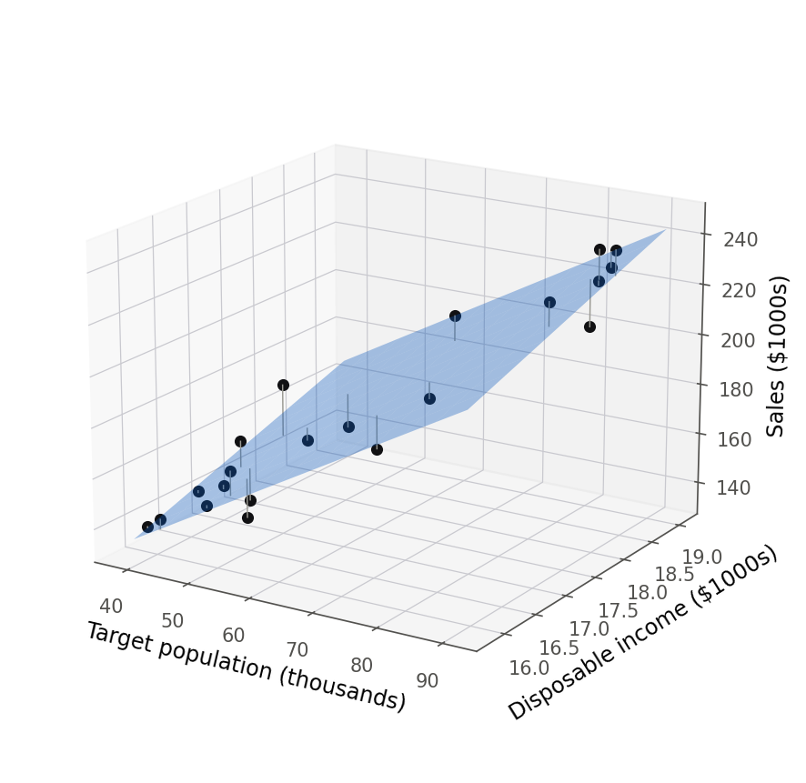
Figure 2:The Dwaine fit is a plane, not a line. Walking in the target-population direction with income held fixed climbs the plane at rate 1.45; walking in the income direction with population held fixed climbs it at rate 9.37. The two partial slopes are the two tilts of this one surface.
8.2 The limits of “holding the others fixed”
Intuition
“Holding the other predictors fixed” is the correct interpretation, and it is also where careful people get into trouble. The phrase is a statement about the arithmetic of the fitted plane: it is always true that the coefficient is the plane’s tilt in one direction with the other coordinates pinned. The trouble is that the sentence quietly promises something the data may not support, that you could actually find, or create, two cities identical in every predictor but one. When predictors move together, that promise is fiction.
Look again at the Dwaine predictors. Target population and disposable income have a correlation of 0.78. Cities with many young families are systematically different in income from cities with few. So “two cities with the same target population but different income” describes a thinner slice of reality than it sounds, and “hold population fixed and push income far” can walk you clean off the cloud of cities that ever existed. The coefficient is still computable and still meaningful as a description of the fitted surface. What weakens is the causal daydream that you could intervene on one predictor and leave the others undisturbed.
The mechanism: a coefficient depends on its companions
A coefficient is not a property of a predictor. It is a property of a predictor and the company it keeps. Add or remove another predictor and the coefficient can move, sometimes a little, sometimes enough to change sign. Figure 3 shows the Dwaine income story both ways: the steep marginal slope when income stands alone, and the gentler partial slope once population is accounted for.
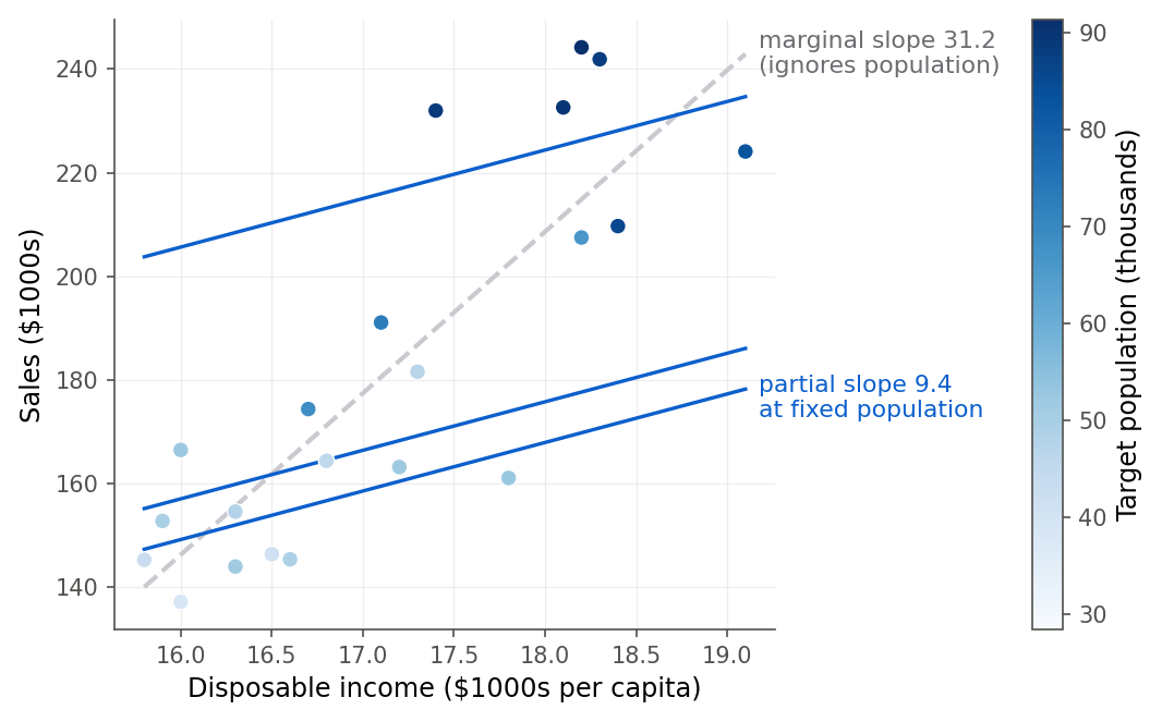
Figure 3:Two answers to “how does income relate to sales.” The steep dashed line ignores population and reports slope 31.17. Within groups of cities that share a population level (same color), the income slope is much gentler, near the partial slope 9.37. The difference is the population that rides along with income in the raw data.
When “holding fixed” describes empty space
The deeper limit is geometric. Holding population fixed and varying income traces a line across the (targtpop, dispoinc) floor. If the data cloud is a tilted ellipse, because the two predictors are correlated, then most of that line lies outside the cloud. The model will still return a fitted value there, but it is extrapolating into a region where no city has ever been observed, and no data constrain the answer. We return to this in 8.7 Two dangers: hidden extrapolation and lurking variables with a picture; for now, hold the warning: a coefficient can be perfectly estimated and still describe a comparison you can never actually make.
The widget below does the holding fixed for you, one population level at a time, so you can watch the gentle partial slope and the steep marginal slope stop looking like rivals.
Slice the fitted plane at one target population and slide that population up and down. The partial slope stays 9.37 while the marginal line, slope 31.17, only traces where those slices sit.
8.3 Extra sums of squares
Intuition
We need a way to ask “how much does a predictor add?” that does not depend on staring at a coefficient. The natural measure is how much unexplained variation a predictor removes when it joins a model that already has the others. Fit the model without the predictor and record its error sum of squares; add the predictor and record the new, smaller error sum of squares; the drop is the predictor’s extra sum of squares (Definition 8.3). It is the variation that only this predictor could mop up, once the others have done their part.
Two facts make this work. First, adding a predictor can never make the error sum of squares larger (we prove this below), so the drop is never negative. Second, the total variation in does not depend on the model, so a smaller means a larger : the extra sum of squares is variation moved from the “unexplained” column to the “explained” column.
A picture makes the “only this predictor could mop up” idea concrete. Think of the response’s variation as a target, and each predictor as a circle that covers the part it can explain. When two predictors are correlated, their circles overlap, and the shared piece can be credited to only one of them: whichever entered the model first. The extra sum of squares of the second predictor is just its own crescent, the part of its circle that the first predictor’s circle did not already cover. Figure 5 draws this for the body-fat predictors we work with next.
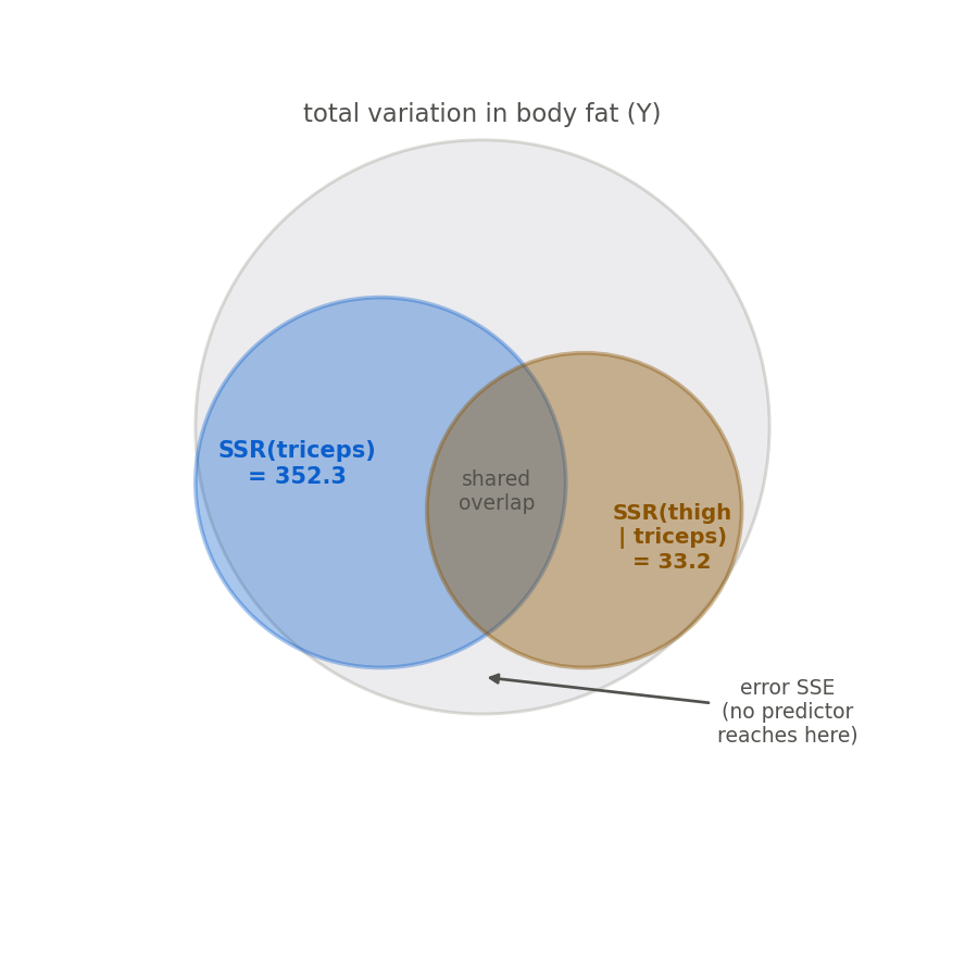
Figure 5:Extra sum of squares as overlapping circles. Triceps enters first and claims the whole shared overlap, so thigh, entering second, gets credit only for its own crescent (33.2), not the larger region it shares with triceps. This is why a later predictor’s extra sum of squares is small when the predictors overlap, and why reordering them changes the split.
Formula
For a model already containing a set of predictors, write for its error sum of squares. The extra sum of squares of given is defined in Definition 8.3.
is the error sum of squares of the model with only.
is the error sum of squares once is added.
The two right-hand expressions are equal because is the same total for both models (3.6 The analysis of variance approach), so any drop in is an equal rise in .
In words: is the extra explained variation you buy by adding to a model that already has . The vertical bar reads “given” or “adjusted for.”
Extra sums of squares chain into a decomposition of the total regression sum of squares. Adding predictors one at a time,
which is exactly what the sequential (Type I) ANOVA table prints, one row per predictor in the order you list them. Because the order is a choice, so is the split: reorder the predictors and the pieces change, though their total does not.
Derivation (adding a predictor cannot increase SSE)
Proof. Let the reduced model use the predictors in a set and the full model use together with one more predictor, so the full model’s columns span a larger space. By 7.2 The geometry of least squares, the fitted vector is the orthogonal projection of onto the column space of the design matrix, and is the squared distance from to that space. Every fitted vector the reduced model can produce is also available to the full model (set the extra coefficient to zero), so the full model’s column space contains the reduced model’s. Projecting onto a larger subspace lands at least as close to :
Therefore , with equality only when the added predictor buys nothing (its fitted contribution is already in the reduced space).
R and Python
The classic worked example is not Dwaine but the ALRM body-fat data: 20 men, percent body fat measured by underwater weighing, against three tape-measure predictors, triceps skinfold, thigh circumference, and midarm circumference. It is built for this section because the predictors overlap heavily, so order matters a lot.
Figure 6 draws the decomposition as a stacked bar: the total variation in body fat split into the sequential pieces plus the leftover error.
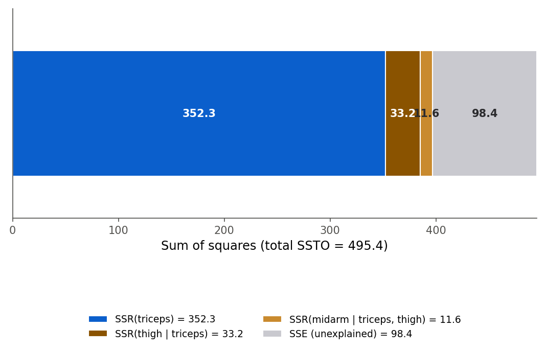
Figure 6:The total variation in body fat, split by sequential extra sums of squares. The first predictor claims the lion’s share; each later predictor adds less because the tape-measure predictors overlap. The rightmost segment is the variation no predictor explained.
8.4 The general linear test
Intuition
Extra sums of squares measure how much a predictor adds; now we ask whether that addition is more than noise would produce. The tool is a comparison of two models, one reduced (without the terms in question) and one full (with them). If the extra terms are worthless, the full model’s error sum of squares will be only trivially smaller than the reduced model’s, a drop no bigger than random scatter would give. If the extra terms matter, the drop will be large relative to the noise level. The general linear test (Definition 8.5) turns “large relative to noise” into a single statistic.
Formula
Let the full model have on degrees of freedom and the reduced model on , where the reduced model is the full model with some coefficients forced to zero. The general linear test statistic and its null distribution are stated in Theorem 8.6.
is the extra sum of squares explained by the terms the reduced model dropped: variation the full model can account for and the reduced model cannot.
is the number of coefficients set to zero under the reduced model, call it .
The denominator is the full model’s estimate of .
In words: is the extra variation explained per dropped coefficient, measured in units of the noise variance. Under the reduced model (the dropped coefficients really are zero) with normal errors, , and a large is evidence against the reduced model. We reject the reduced model when exceeds the upper critical value, equivalently when its -value is small.
Derivation (the test statistic and its distribution)
Proof. Write and for the fitted vectors of the full and reduced models. By 7.2 The geometry of least squares each is the orthogonal projection of onto a column space, and the reduced space is a subspace of the full space. Split the reduced model’s residual through the full fit:
The full residual is orthogonal to the entire full column space, and lies inside that space, so the two pieces are perpendicular. Pythagoras gives
so the numerator sum of squares is the squared length of the extra-fit vector, which lives in a subspace of dimension . That is where its degrees of freedom come from. Figure 7 draws this right triangle.
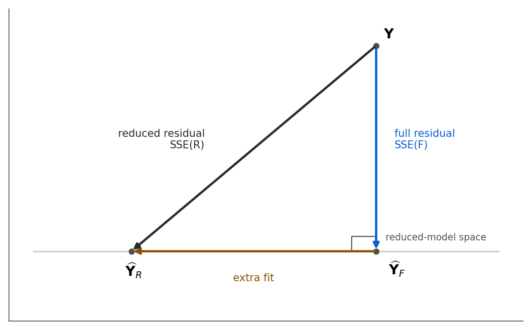
Figure 7:The general linear test is Pythagoras. The reduced residual (hypotenuse, SSE(R)) splits into the full residual (long leg, SSE(F)) and the extra-fit vector (short leg), which meet at a right angle. The test compares the short leg’s squared length, per dropped coefficient, to the noise level.
The distributional claim needs one more layer. Under the reduced model with normal errors, the two perpendicular pieces are independent, and each squared length divided by is a chi-square: and . Dividing each chi-square by its degrees of freedom and taking the ratio gives an variable. The independence and chi-square facts rest on the normal-theory geometry of projections built in 7.3 The hat matrix. The full argument uses Cochran’s theorem on quadratic forms, which is beyond the matrix algebra this book proves. So we take those two distributional facts on the authority of that geometry, and verify the whole machine numerically below. The ALRM text, Chapter 7, gives the quadratic-form details for the reader who wants them.
Tests on a subset of coefficients
The savings data give a clean subset test, and they carry the second running thread of this chapter.
In Chapter 4 you used these 50 countries to study correlation and its traps (4.2 Correlation and the regression slope); we
now fit them as a multiple regression. The response sr is the aggregate personal savings rate, and
the predictors are the percent of population under 15 (pop15), the percent over 75 (pop75),
per-capita disposable income (dpi), and its growth rate (ddpi). Life-cycle savings theory says
the two dependency measures, pop75 and dpi, might not matter once age structure and growth are
in the model. That is a hypothesis about two coefficients at once, and the general linear test is
built for it.
One coefficient: the test is exactly 
When the reduced model drops a single coefficient (), the general linear test must agree with the -test that software already prints for that coefficient. It does, exactly.
Proof. From 7.4 The sampling distribution of b the estimated variance of is , where is the -th diagonal entry of . The extra sum of squares for dropping the single predictor works out to . Substituting both into the general linear test with ,
So the subset test with one dropped coefficient is the square of the ordinary statistic, and an variable is the square of a variable. The two tests are one test.
Before you trust any single row of a sequential table, promote and demote the predictors yourself and watch re-decide whether the newest one earned its place.
Let the body-fat predictors in one at a time, in any of the six entry orders, and watch each extra sum of squares and its general linear test F* change while the total SSR does not.
8.5 Added-variable plots
Intuition
A coefficient is a single number; sometimes you want to see the partial relationship it summarizes. The obstacle is that you cannot simply plot against , because that picture mixes in every other predictor. The added-variable plot (Definition 8.8), also called a partial regression plot, removes the other predictors from both axes first, then plots what is left.
Here is the recipe. To see the partial effect of : regress on all the other predictors and keep the residuals , the part of the others do not explain. Regress on all the other predictors and keep the residuals , the part of the others do not explain. Now plot against . Both axes have been purged of the other predictors, so the plot shows the relationship between and that is genuinely new. Its slope is exactly the multiple regression coefficient , a fact we prove below, so the plot is a picture of the very number in the coefficient table.
The one rule people break is forgetting to clean the horizontal axis: they residualize but then plot it against the raw predictor. Figure 9 lays out the three steps so both axes get the same treatment.
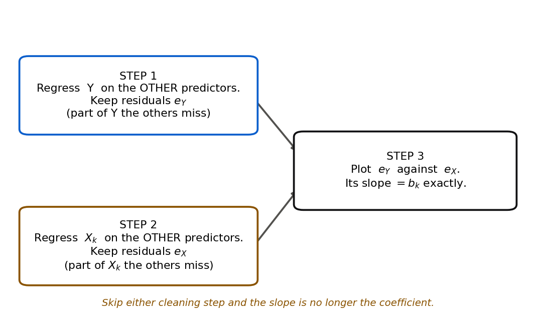
Figure 9:The added-variable plot in three steps. Both axes must be purged of the other predictors before plotting, not just the response. Clean only one axis and the slope is no longer the coefficient, which is the mistake Try it 8.5 walks through.
Formula
For predictor in a model whose other predictors are collected as ,
and the added-variable plot is the scatter of against . The least-squares slope of that scatter equals , the full-model coefficient on .
is the response with the other predictors’ explanation removed.
is predictor with the other predictors’ explanation removed, its unique part.
The slope of on is ; the scatter around the line shows how cleanly ’s unique part predicts ’s unmatched part.
Derivation (the added-variable slope equals )
Proof (Frisch-Waugh, two-predictor case). Take the full model and let play the role of “the other predictor” while we build the added-variable plot for . Split into its projection onto and the leftover: , where by construction. Substitute into the fitted equation and group the terms that live in :
Now form by removing the part of , that is, projecting onto the orthogonal complement of . The first group vanishes under this projection. The term is already orthogonal to , so it survives untouched. The full residual is orthogonal to , hence to , so it survives too. Therefore
Finally regress on through the origin (both residual vectors have mean zero). The slope is
because : the full residual is orthogonal to and to , hence to . The added-variable slope is exactly the multiple regression coefficient. The same argument works with any number of other predictors in place of .
R and Python
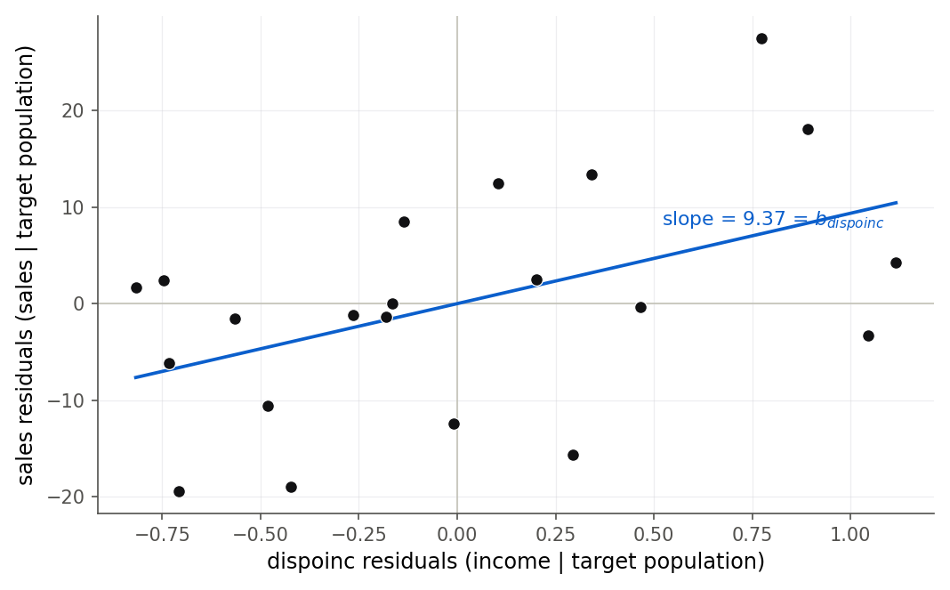
Figure 10:The added-variable plot for income, with target population purged from both axes. Its slope is the multiple regression coefficient 9.37 exactly. The upward tilt confirms income adds information beyond population; the scatter shows how much.
An added-variable plot can also reveal the opposite, a predictor with almost nothing left to add.
Figure 11 shows the plot for growth rate ddpi in the savings model, whose partial
slope is a positive but gentle 0.41.
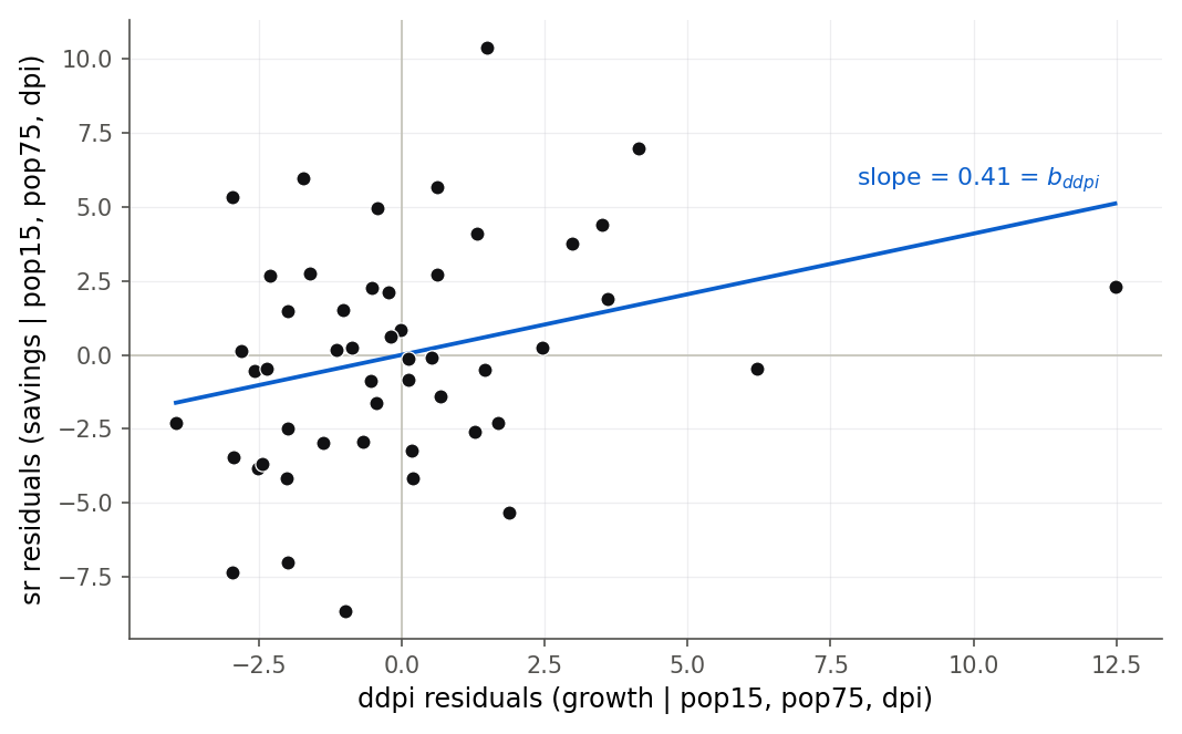
Figure 11:The added-variable plot for income growth in the savings model. The gentle upward slope, 0.41, is the partial effect of growth on savings once age structure and income are accounted for. The wide scatter is why the effect, though real, is only marginally significant.
Rather than take the recipe on faith, pull the cleaning slider below and watch the marginal slope turn into the coefficient in front of you.
Remove what target population explains from both axes, a little at a time, and watch the slope travel from the marginal 31.17 to the added-variable slope 9.37, which is exactly the coefficient on dispoinc.
8.6 , adjusted , and standardized coefficients
Intuition
We can now test which predictors belong; the next job is to summarize a whole model in one number and compare models of different sizes fairly. is the fraction of the response’s variation the model explains, and it has one seductive flaw: it never goes down when you add a predictor, even a column of random noise. That makes it useless for comparing models of different sizes, because the biggest model always wins. Adjusted (Definition 8.10) fixes this by charging rent for each predictor: it goes up only if the new predictor explains more than an average predictor’s worth of noise would. Standardized coefficients (Definition 8.11) solve a different problem: raw coefficients live in different units (dollars, thousands of people, percents), so you cannot compare their sizes; putting everything in standard-deviation units makes the comparison fair.
Formula
is the total variation in , fixed regardless of the model.
compares raw sums of squares; compares them per degree of freedom, so adding a parameter (raising ) is penalized through the factor .
A standardized coefficient is , the coefficient you get by fitting the regression on variables first rescaled to have standard deviation one.
In words: measures explained fraction, measures explained fraction after paying for model size, and measures effect size in standard deviations, so different predictors can be ranked on one scale.
Derivation ( never falls; can)
Proof. By the monotonicity result of 8.3 Extra sums of squares (Theorem 8.4), adding a predictor cannot raise , and does not depend on the model. Hence cannot rise, so cannot fall: every added predictor leaves equal or higher, which is why alone cannot choose a model. Adjusted behaves differently because it uses . Adding a useless predictor lowers by a little but also lowers the divisor by one; if the shrinkage in is smaller than the shrinkage in demands, rises and falls. So can go down when a predictor does not earn its degree of freedom, which is exactly the behavior we want from a model-size-aware measure.
Figure 13 makes this concrete: starting from the real savings model, we add columns of pure random noise one at a time and watch climb while sags.
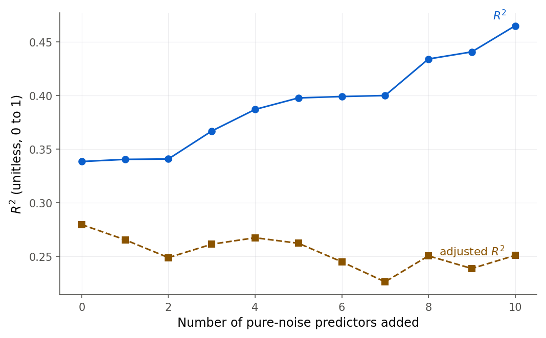
Figure 13:Adding pure noise predictors to the savings model. R-squared (upper curve) rises with every junk column, because it never falls when a predictor is added. Adjusted R-squared (lower curve) drifts down, correctly reporting that the noise columns are not worth their degrees of freedom.
R and Python
Figure 14 ranks the four standardized coefficients on one axis, which the raw coefficients, living in incompatible units, could never share.
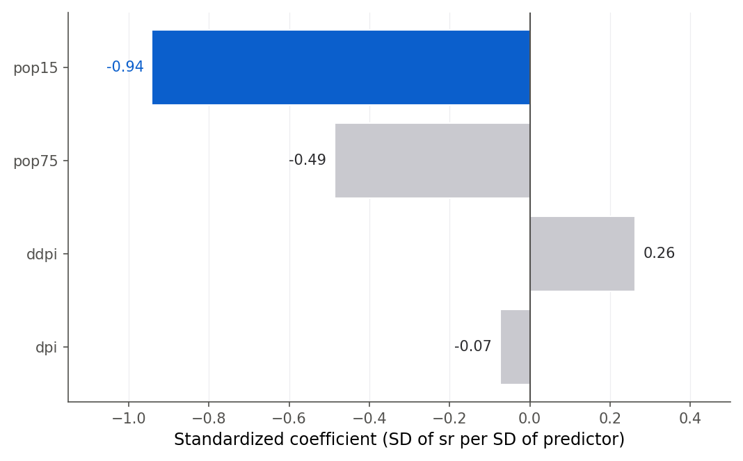
Figure 14:The savings coefficients on a common standard-deviation ruler. Young-population share (pop15) has by far the largest standardized effect, and it is negative; income (dpi) has almost none. Only after standardizing can predictors in percent and in dollars be compared this way.
8.7 Two dangers: hidden extrapolation and lurking variables
Intuition
Two failures deserve their own section because they are invisible in the coefficient table and fatal to a conclusion. The first is hidden extrapolation (Definition 8.13): predicting at a combination of predictor values that is inside the range of each predictor separately but outside the region where they occur together. The second is the lurking variable (Definition 8.14): an omitted predictor that, if included, would move or reverse the coefficients you reported.
Hidden extrapolation
With one predictor, extrapolation is easy to police: stay inside the observed range of . With several predictors, the observed region is not a box but a cloud, usually a tilted one because predictors are correlated. A query point can sit inside every predictor’s own range and still fall far outside the cloud. Figure 15 shows the Dwaine case: a city with target population 75 and disposable income 16 is unremarkable on each axis alone, yet no real city combines a population that large with income that low, so a prediction there is an extrapolation the one-variable ranges would never flag.
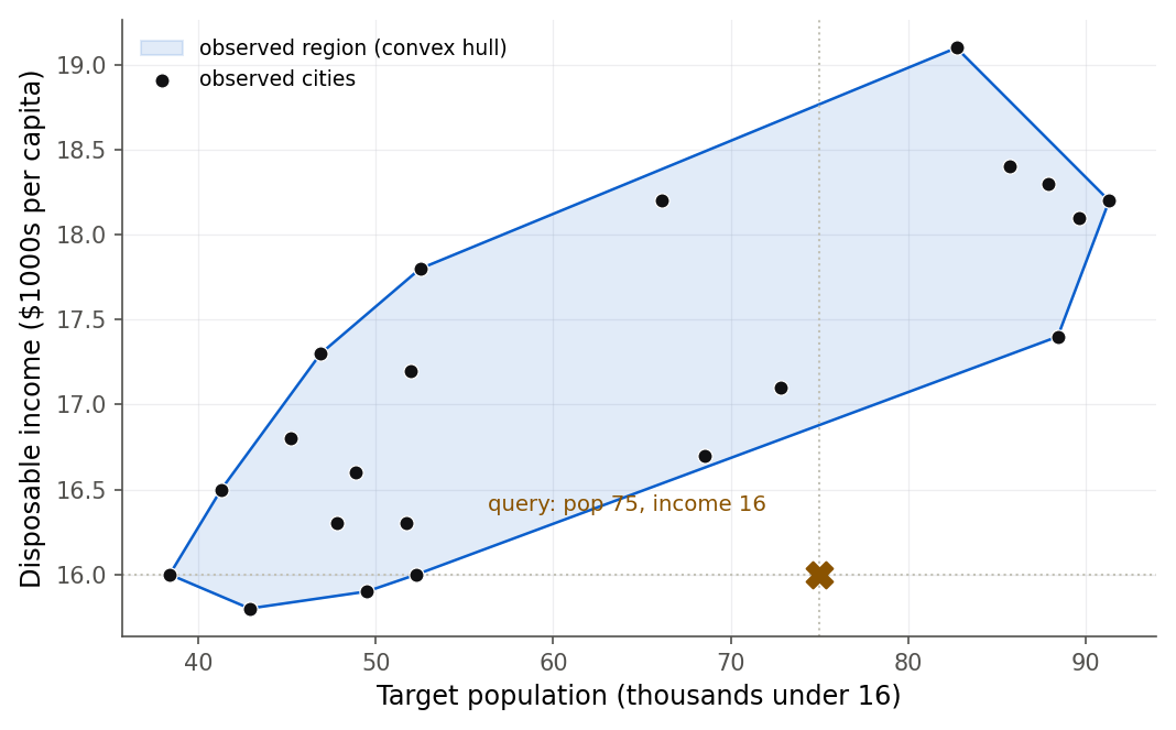
The practical check is to ask whether a query point lies within the joint region of the data, not merely within each margin. Chapter 9 makes this rigorous with the hat matrix: the leverage value of 7.3 The hat matrix measures how far a point sits from the center of the predictor cloud, and a new point whose leverage value would exceed the observed ones is a hidden extrapolation.
Lurking variables
A regression can only adjust for the predictors you give it. If an important variable is missing and it correlates with both the response and an included predictor, the coefficient you report absorbs the missing variable’s influence and can be badly wrong, even reversed. This is the multiple regression version of the correlation-is-not-causation warning from 4.2 Correlation and the regression slope, and it is why an observational coefficient is always provisional: some unmeasured factor might be doing the work.
“Even reversed” sounds like an exaggeration until you see it. Figure 16 shows the mechanism on a schematic dataset. Ignore the lurking variable and the points march up from left to right, so the slope looks positive. Color the points by the hidden group and each group tips the other way: within any single group the slope is negative. A model that never saw the group reports the upward trend and gets the sign exactly backwards.
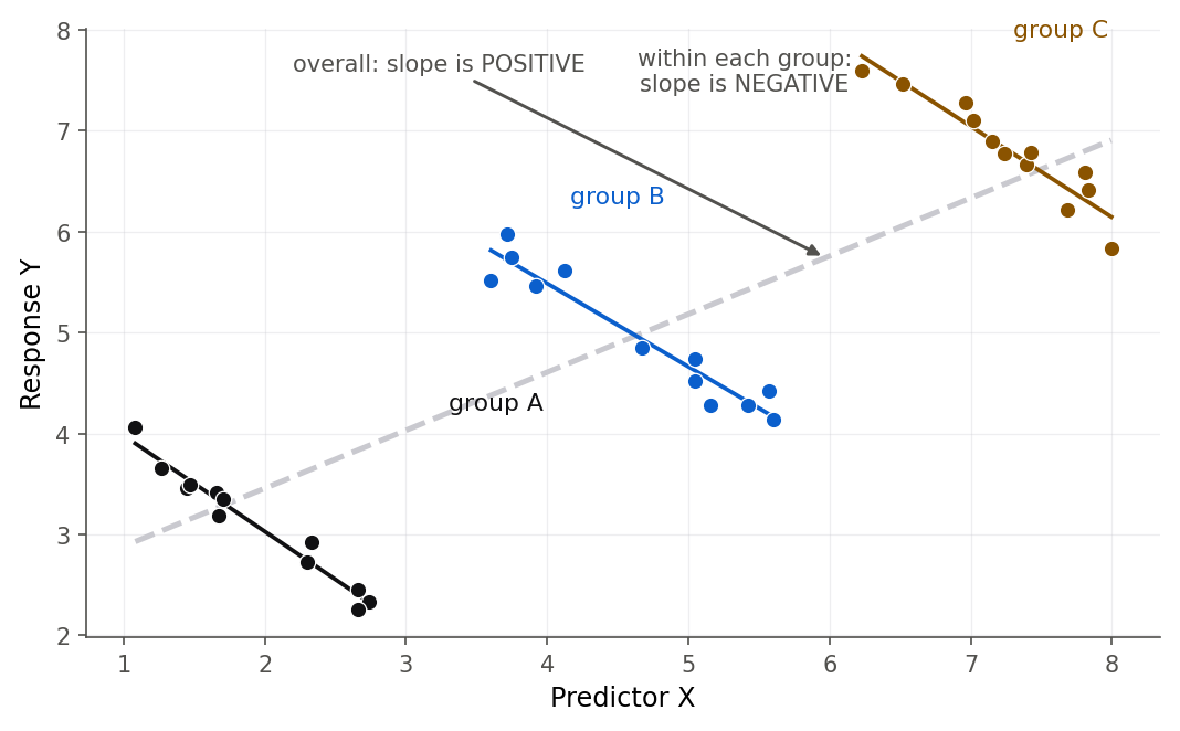
Figure 16:A lurking variable can flip a slope’s sign. The dashed overall line slopes up because the groups sit at different heights; the solid within-group lines all slope down. If the group is a variable you never measured, your fitted coefficient reports the up-slope and misses the true down-slope entirely.
The honest posture is to name the lurking variables you can think of and admit the ones you cannot. In the Dwaine study, local competition, the age of each studio, and regional advertising are all plausibly related to both sales and the city characteristics; none is in the model, so each partial slope is “the best we can say from these three columns,” not a final truth. No amount of arithmetic inside a fixed set of predictors can rule out a variable you never measured.
8.8 Chapter summary
You can now take a fitted multiple regression and do the work that matters after the fit. You can read each coefficient as a partial slope, stating in words the controlled comparison it makes and the exact phrase “holding the other predictors fixed,” and you can explain why that phrase weakens when predictors are correlated and can describe a region with no data. You can compute extra sums of squares and read a sequential ANOVA table as a decomposition of . You can run the general linear test for one coefficient or a group, derive its statistic from the Pythagorean split of nested models, and show it collapses to for a single coefficient. You can build an added-variable plot and prove its slope is the multiple regression coefficient. You can compute , adjusted , and standardized coefficients, and explain why only the last two are safe for comparing models or effects. And you can spot the two dangers that a coefficient table hides: hidden extrapolation in the joint predictor space and the lurking variable no model ever measured.
Key results at a glance
| Result | Statement or formula | Valid when |
|---|---|---|
| Partial slope (Definition 8.1) | is the change in per unit of , other predictors held fixed | multiple regression model |
| Extra sum of squares (Definition 8.3) | any nested pair of models | |
| Monotonicity of SSE (Theorem 8.4) | , so | reduced predictors a subset of the full |
| General linear test (Theorem 8.6) | normal errors, reduced model true | |
| One-coefficient identity (Theorem 8.7) | dropping a single coefficient () | |
| Added-variable slope (Theorem 8.9) | slope of on equals | any multiple regression (Frisch-Waugh) |
| monotonicity (Theorem 8.12) | never falls as predictors are added; can | comparing nested models |
| Adjusted (Definition 8.10) | comparing models of different size | |
| Standardized coefficient (Definition 8.11) | ranking effects across different units |
Key terms
partial slope, multiple linear regression model, extra sum of squares, sequential (Type I) ANOVA, general linear test, full model, reduced model, added-variable plot, coefficient of determination (), adjusted , standardized coefficient, hidden extrapolation, lurking variable, multicollinearity.
You should now be able to
Read each coefficient as a partial slope, with its units and the phrase “holding the other predictors fixed.”
Explain why “holding fixed” weakens under correlated predictors and can describe a region with no data.
Compute an extra sum of squares and read a sequential ANOVA table as a decomposition of .
Run the general linear test for one coefficient or a group, and show it reduces to when .
Build an added-variable plot and prove its slope equals the multiple regression coefficient.
Compute and contrast , adjusted , and standardized coefficients, and say why never falls when a predictor is added.
Spot hidden extrapolation in the joint predictor space and explain how a lurking variable can flip a coefficient’s sign.
Where this fits. In the workflow spine of The modeling workflow this chapter is mostly USE: it takes the fit that Chapter 7 produced for Dwaine in matrix form and turns it into interpretation, tests, and honest caveats, with the general linear test also serving FIT by deciding which terms belong. Chapter 7 gave the estimator and its variance; this chapter gave the reasoning that makes an estimate a claim. What we deferred is the CHECK stage: whether any single case is quietly running the fit, and whether the model’s assumptions hold at all. That is Chapter 9’s job. It returns to the savings data, singling out Libya as the case that bends the fit and Zambia as a large-residual outlier, and builds the influence diagnostics (9.3 Influence: which points actually change the fit) and the leverage statistic that 9.1 Leverage values and the hat matrix points to, which together decide how much of this chapter’s confidence survives contact with real data. The general linear test you learned here is the testing engine that Chapter 11 reuses for categorical predictors and interactions (11.1 From categories to numbers: indicator coding) and Chapter 12 for variable selection (12.2 Choosing among models: selection criteria), neither re-deriving it.
8.9 Frequently asked questions
Q1. Why is the multiple regression coefficient on income so different from the simple-regression slope? Because they answer different questions. The simple slope 31.17 compares cities that differ in income and lets population differ along with it; the partial slope 9.37 compares cities that differ in income but share population. When predictors are correlated, the two questions have different answers, and only the partial slope earns the phrase “holding population fixed.”
Q2. Does “holding the other predictors fixed” mean I can intervene on one predictor and expect that coefficient’s change? No. The coefficient describes a comparison across cases that already differ, not the effect of an action. With observational data, and especially with correlated predictors or a lurking variable, acting on a predictor need not reproduce the observed association. The coefficient is a description of the fitted surface, not a promise about interventions.
Q3. The sequential ANOVA gives different sums of squares when I reorder the predictors. Which order is right? None is uniquely right; the order is a choice about what “given the others” means. The first predictor gets its full simple-regression sum of squares, each later one gets only what it adds beyond those before it. The pieces always total the same . If you want each predictor adjusted for all the others at once, use its -test (or the general linear test dropping just that predictor), which does not depend on order.
Q4. When should I use the general linear test instead of just reading statistics? Use it whenever you want to test several coefficients at once, such as “do these two predictors together add anything.” A group of individually non-significant ’s does not tell you whether the group as a whole matters, because the predictors may share their explanatory power; the general linear test asks the joint question directly. For a single coefficient, the general linear test and the -test are identical ().
Q5. Why does always go up when I add a predictor, even a useless one? Because adding a predictor can only lower (or not change) , and is fixed, so can only rise. That is exactly why cannot be used to choose between models of different sizes; use adjusted , which penalizes each added parameter, or a formal test.
Q6. My added-variable plot slope matches the coefficient exactly. Is that a coincidence? No, it is a theorem (Frisch-Waugh). Removing the other predictors from both the response and the target predictor, then regressing the leftovers, reproduces the full-model coefficient exactly. That is what makes the added-variable plot a faithful picture of the coefficient rather than a rough sketch.
Q7. All three body-fat coefficients are non-significant, yet the overall is highly significant. How can the model be useful if no single predictor is? This is the fingerprint of multicollinearity. The three tape-measure predictors overlap so much that no one of them adds much given the other two, so each individual is small; but together they explain body fat well, so the overall is large. The predictors are substitutes, not independent contributors. Chapter 12 takes up this multicollinearity theme on a larger body-fat study and measures the overlap with the variance inflation factor.
8.10 Practice problems
(A) State in one sentence what the Dwaine coefficient 1.4546 on
targtpopmeans, naming its units and what is held fixed.(A) Explain the difference between the simple-regression slope of
salesondispoinc(31.17) and the multiple regression coefficient (9.37). Which holds population fixed?(A) Define the extra sum of squares in words, and explain why it can never be negative.
(A) A reduced model drops three predictors from a full model. State the numerator degrees of freedom of the general linear test comparing them.
(A) Why does never decrease when a predictor is added? Answer using the identity .
(A) A colleague reports that adjusted fell when they added a variable, and concludes they made an error. Are they right? Explain.
(A) In your own words, what does an added-variable plot put on each axis, and why is neither axis the raw variable?
(A) Give an example, in the Dwaine context, of a lurking variable that could distort the income coefficient, and say why it would matter.
(A) Explain why a query point can be a hidden extrapolation even when each predictor value is inside its own observed range.
(A) All three body-fat coefficients are individually non-significant but the overall is highly significant. Explain how both can be true.
(B) Prove that adding a predictor to a model cannot increase (Theorem 8.4), using the projection characterization of least squares from 7.2 The geometry of least squares.
(B) Show that is equivalent to , citing which quantity is model-independent.
(B) Derive the Pythagorean identity for nested models, stating where orthogonality is used.
(B) Starting from and , prove that the general linear test with gives (Theorem 8.7).
(B) Prove that the slope of the added-variable plot for equals the full-model coefficient , in the two-predictor case (Theorem 8.9, Frisch-Waugh).
(B) Derive from the definition , and explain when adding a predictor lowers it.
(B) Show that the standardized coefficient satisfies by relating the regression on standardized variables to the regression on raw variables.
(B) Explain why reordering predictors changes the sequential sums of squares but never changes their total or the full-model coefficients. Tie your answer to which quantities the order affects.
(B) The general linear test for the overall regression compares the full model to the intercept-only model. Show that its equals with .
(C) Fit the Dwaine model in R or Python and reproduce , , and the residual standard error. Confirm from the residuals.
(C) On
bodyfat3.csv, print the sequential ANOVA in both predictor orders (triceps-then-thigh and thigh-then-triceps) and report how and differ. Explain the difference.(C) Run the general linear test dropping
pop75anddpifrom the savings model, first with the built-in model comparison and then by hand from the two error sums of squares. Confirm they agree and report and its -value.(C) For the savings model, verify for the single predictor
ddpi: compute the general linear test droppingddpiand compare to the square ofddpi’s statistic.(C) Build the added-variable plot for
pop15in the savings model. Report the slope, confirm it equals the full-model coefficient onpop15, and describe the scatter.(C) Add three columns of standard normal noise (seed
4210) to the savings data, refit with the extra columns, and report how and adjusted change. Which one behaves sensibly?(C) Standardize the Dwaine variables and refit; report the two standardized coefficients and say which predictor has the larger standardized effect. Does the ranking match the raw statistics?
(C) Predict Dwaine sales at target population 75 and income 16, and separately at the sample means. Argue from Figure 15 which prediction you would trust and why.
(C) Fit the full three-predictor body-fat model and report all three statistics and the overall . Explain, using the correlations among the predictors, why the individual and joint verdicts disagree.
(B) A student claims that because always, adding any predictor always improves the model. Explain precisely what “improves” can and cannot mean here, distinguishing , , adjusted , and out-of-sample prediction.
(C) Using the Dwaine model, compute a 95% confidence interval for mean sales and a 95% prediction interval for a new city’s sales at target population 65.4 and income 17.6. Explain in one sentence why the prediction interval is wider, citing 3.5 Prediction interval for a new observation.
8.11 Exam practice
These five questions are written in the style of the course exams: each one asks you to explain your reasoning in full sentences, not just to produce a number. Read the output, decide what it says, and write the argument you would want a grader to read. Work each one before opening its model answer.
EP 8.1. The four-predictor savings model is fit to the 50 countries, and R prints the coefficient table below.
            Estimate Std. Error t value Pr(>|t|)
(Intercept)  28.5661     7.3545  3.8842   0.0003
pop15        -0.4612     0.1446 -3.1885   0.0026
pop75        -1.6915     1.0836 -1.5610   0.1255
dpi          -0.0003     0.0009 -0.3618   0.7192
ddpi          0.4097     0.1962  2.0882   0.0425
Interpret the coefficient on pop15 as a partial slope, giving its units and the exact phrase for
what is held fixed. Then, using the value and -value, explain whether pop15 is
distinguishable from zero at the 5% level. Finally, a classmate reads the near-zero dpi coefficient
and concludes that disposable income has no relationship with the savings rate; explain
in full sentences why that conclusion overreaches.
Model answer
The coefficient -0.4612 on pop15 is a partial slope: comparing two countries that share the same
values of pop75, dpi, and ddpi, the one whose share of population under 15 is one percentage
point higher is predicted to have a savings rate about 0.46 percentage points lower. The units are
percentage points of savings rate per percentage point of young-population share, and the phrase that
earns the interpretation is “holding pop75, dpi, and ddpi fixed.” Because with a
-value of 0.0026, far below 0.05, pop15 is clearly distinguishable from zero at the 5% level;
the data give strong evidence that its partial slope is not zero. The classmate overreaches on two
counts. First, the coefficient is tiny in size mainly because dpi is measured in raw dollars, so a
one-dollar change is a minuscule move and its per-dollar effect is naturally small; size on a raw
scale is not the same as importance, which is why we standardize before ranking effects. Second, and
more basic, the coefficient measures the partial effect of income given the other three predictors,
not income’s total relationship with saving. A large simple correlation between dpi and the savings
rate could still exist and be absorbed by pop15 and pop75, which are themselves correlated with
income. The honest statement is that income adds little once age structure and growth are in the
model, not that income is unrelated to saving.
A weak answer reports “not significant” or “significant” without stating the controlled comparison
and units behind pop15, and accepts the classmate’s leap from a small coefficient to “no
relationship” without separating raw scale from importance or partial effect from total association.
EP 8.2. A student fits the three body-fat predictors in two different orders and prints the sequential (Type I) ANOVA table each time.
Response: bodyfat        (order: triceps, thigh, midarm)
          Df Sum Sq Mean Sq F value    Pr(>F)
triceps    1 352.27  352.27 57.2768 1.131e-06
thigh      1  33.17   33.17  5.3931   0.03373
midarm     1  11.55   11.55  1.8773   0.18956
Residuals 16  98.40    6.15
Response: bodyfat (order: thigh, triceps, midarm)
Df Sum Sq Mean Sq F value Pr(>F)
thigh 1 381.97 381.97 62.1052 6.735e-07
triceps 1 3.47 3.47 0.5647 0.46330
midarm 1 11.55 11.55 1.8773 0.18956
Residuals 16 98.40 6.15The student writes: “Thigh gets a sum of squares of 381.97 in the second table but only 33.17 in the first. The same variable cannot have two different sums of squares, so one of these tables must be a software error.” Evaluate this claim, and explain in full sentences what the two thigh numbers actually represent.
Model answer
The student is wrong; both tables are correct, and they are not reporting the same quantity. A sequential ANOVA table gives each predictor the extra sum of squares it earns given the predictors listed before it, so the row for a variable depends on its position. In the first table thigh enters second, so its row is : the variation thigh explains after triceps has already claimed everything the two share. In the second table thigh enters first, so its row is : the variation thigh explains on its own, including the large piece it shares with triceps. The two numbers differ precisely because triceps and thigh are strongly correlated, so most of thigh’s marginal explanatory power overlaps triceps and gets credited to whichever predictor enters first. Nothing is inconsistent: both tables have the same residual sum of squares 98.40 and the same total, and both give midarm the same last-place row 11.55 because in both orders midarm enters after the other two. The lesson is that a Type I sum of squares answers “given the earlier predictors,” not “for this predictor alone,” so reordering is expected to move the middle rows while leaving the total and the full-model coefficients unchanged.
A weak answer just says “order matters” without naming that the two numbers are versus , and misses that the overlap exists because the predictors are correlated, which is the reason the split changes.
EP 8.3. In the savings model you want to know whether the two economic predictors, dpi and
ddpi, can be dropped once the two demographic predictors pop15 and pop75 are in the model. The
model comparison prints:
Model 1: sr ~ pop15 + pop75
Model 2: sr ~ pop15 + pop75 + dpi + ddpi
  Res.Df    RSS Df Sum of Sq     F  Pr(>F)
1     47 726.17
2     45 650.71  2    75.455 2.609 0.08471
State the null and alternative hypotheses this test evaluates and your decision at the 5% level. Then,
recalling from the full-model summary in EP 8.1 that dpi has () while ddpi
has (), explain in full sentences why it would be a mistake to react to this
non-significant joint test by dropping both dpi and ddpi.
Model answer
The test compares the reduced model, which forces both economic coefficients to zero, against the
full model that keeps them. The null hypothesis is that
together, and the alternative is that at least one of them is nonzero. The statistic is
on 2 and 45 degrees of freedom, with a -value of
0.085. At the 5% level this is not significant, so the joint test does not reject the reduced model:
the two economic predictors do not clearly improve the fit as a pair. It would still be a mistake to
drop both. The joint test asks a single yes-or-no question about the two coefficients at once, and its
answer is diluted by dpi, which contributes almost nothing (its individual is -0.36). But
ddpi on its own is individually significant at the 5% level (, ), meaning
growth in disposable income does add information beyond the demographics. Averaging a useful predictor
with a useless one can push a joint below significance even though one member of the pair belongs
in the model. The sensible move is to drop dpi alone and re-examine ddpi, not to discard both on
the strength of one blurred joint test.
A weak answer stops at “, so drop both,” treating the joint test as if it licensed
dropping each predictor individually, and never notices that ddpi is significant on its own.
EP 8.4. For the savings model, the added-variable plot for pop15 is built by residualizing both
the response and pop15 on the other three predictors, and its slope is computed.
AV slope pop15 = -0.4612 full coef pop15 = -0.4612Explain why the added-variable plot slope must equal the full-model coefficient, naming the result
that guarantees it. Then explain what would change if a student residualized only the response sr on
the other predictors but plotted those residuals against the raw pop15 values instead of the
residualized pop15: would the slope still be -0.4612, and what quantity would that botched slope
represent?
Model answer
The added-variable plot puts , the response with the other three predictors removed, on the
vertical axis, and , pop15 with the same three predictors removed, on the horizontal axis. By
the Frisch-Waugh result (Theorem 8.9), the least-squares slope of on equals the
full-model coefficient exactly, which is why both numbers print as -0.4612: the
plot is a faithful picture of the coefficient, not an approximation to it. If the student cleans only
the vertical axis and plots against raw pop15, the equality breaks. The horizontal axis still
carries the part of pop15 that overlaps pop75, dpi, and ddpi, so the confounding that the
added-variable plot exists to strip out has only been removed from one axis, not both. The resulting
slope would not be -0.4612 in general, and it would not be the simple regression slope of sr on
pop15 either; it is an uninterpretable hybrid, the slope of a partly-cleaned response on a
not-cleaned predictor, that answers no well-posed question. The discipline of the method is that both
axes must have the same other predictors removed; residualizing one axis and not the other is the
single most common way people break the construction.
A weak answer says only “the slope changes” without explaining that the raw horizontal axis re-mixes the confounding, and without recognizing that the botched slope equals neither the partial slope -0.4612 nor the simple-regression slope.
EP 8.5. Starting from the four-predictor savings model, three columns of pure standard-normal
noise (seed 4210) are added and the model is refit.
model                     R2       adj R2
sr ~ 4 predictors         0.3385   0.2797
sr ~ 4 predictors + 3 noise 0.3980   0.2977
Explain why rose from 0.3385 to 0.3980 even though the three added columns are pure noise. Then explain why this rise is not evidence that the larger model is better, and say what adjusted and out-of-sample prediction each tell you here.
Model answer
, and by the monotonicity of (Theorem 8.12) adding any predictor, useful or useless, can only lower or leave it unchanged, while is fixed because it depends only on the response. So can only rise or stay flat, and here it rose by about 0.06. That rise is an in-sample artifact: with only 50 countries, three random columns can be tuned by least squares to soak up a little of the idiosyncratic wiggle in this particular sample, which lowers even though the columns carry no real signal. It is not evidence of a better model, because never falls when predictors are added and therefore cannot distinguish a real improvement from noise fitting. Adjusted is the honest comparison: it charges a degrees-of-freedom rent through the factor , and here it barely moved, rising only from 0.2797 to 0.2977 against ’s much larger jump, so it does not reward the noise columns the way does. Adjusted is not forced upward, and over many junk columns it drifts down, as Figure 13 shows. Out-of-sample prediction would be the sharpest verdict: on new countries the noise columns carry no signal, so the larger model would predict as well or worse than the four-predictor model, exposing the gain as overfitting.
A weak answer treats the higher as a genuine improvement, or claims adjusted is guaranteed to fall when noise is added; the correct point is that must not fall by construction, while adjusted merely stops rewarding size automatically.
Resumen del capítulo (en español)
Este capítulo trata lo que sigue tras ajustar una regresión múltiple (multiple regression). Retomamos a Dwaine Studios del Capítulo 7, donde resolvimos las ecuaciones normales para obtener , y aprendemos a interpretarlos con honestidad. Un coeficiente de regresión múltiple es una pendiente parcial (partial slope): el cambio en la respuesta media por cada unidad del predictor, manteniendo fijos los demás predictores. Esta frase describe bien la superficie ajustada, pero se debilita cuando los predictores están correlacionados, porque “mantener fijo” puede describir una región sin datos.
El coeficiente cambia según qué otros predictores lo acompañan: la pendiente de sales sobre
dispoinc cae de 31.17 a 9.37 al agregar targtpop, porque el segundo número controla la
población. Definimos las sumas de cuadrados adicionales (extra sums of squares),
, que miden cuánta variación
explica un predictor una vez incluidos los demás, calculadas con los datos de grasa corporal:
.
La prueba lineal general (general linear test) compara un modelo completo con uno reducido mediante
, derivada con el
teorema de Pitágoras para modelos anidados; para un solo coeficiente se reduce a .
Con los datos de ahorro mostramos que pop75 y dpi pueden eliminarse (, ).
Los gráficos de variable agregada (added-variable plots) muestran la relación parcial: su pendiente
es exactamente el coeficiente. Distinguimos también , que nunca baja al agregar predictores, del
ajustado (adjusted), que penaliza el tamaño del modelo, definimos los coeficientes
estandarizados (standardized coefficients) para comparar efectos, y advertimos sobre dos peligros: la
extrapolación oculta (hidden extrapolation) en varias dimensiones y las variables ocultas
(lurking variables) que ningún modelo llegó a medir. El Capítulo 9 revisa estos mismos datos con
diagnósticos de influencia.