Measuring body fat well is a nuisance. The accurate way is to weigh a person underwater
and work out their density, which needs a tank, a technician, and a cooperative subject.
The cheap way is a tape measure. So a natural question follows: can a handful of tape
measurements (waist, chest, thigh, wrist, and the rest) predict the percent body fat that
the underwater weighing gives? A 1985 study recorded both for 252 men, and that dataset,
fat.csv, is the one this chapter works with from start to finish. (This is the larger
252-man study with thirteen measurements, not the three-measurement, twenty-man body-fat
table you met for extra sums of squares in 8.5 Added-variable plots; the two share a “thigh” column
but are different data.)
There is an obvious plan: regress body fat on all thirteen measurements and read off the coefficients. When you do, the model explains about 75 percent of the variation, which sounds like a success. Then you look at the coefficients and something is wrong. The coefficient on weight is negative, as if heavier men had less fat once you hold the other measures fixed. Several predictors that everyone knows matter come out statistically insignificant. Drop one measurement and the others lurch. The problem is that the tape measurements are all measuring roughly the same thing, body size, so they are tangled together. Figure 1 shows just how tangled.
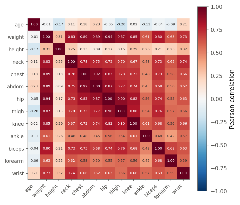
Figure 1:The girth measurements are strongly correlated with one another (weight and hip correlate 0.94, chest and abdomen 0.92). Predictors this redundant carry almost the same information, which is what makes their individual coefficients hard to pin down.
This chapter is about living with too many predictors, most of them redundant. Three questions organize it. First, how do we diagnose and describe the damage that correlated predictors do, using the variance inflation factor? Second, when several models are on the table, how do we choose, using criteria like Mallows and cross-validation that reward prediction rather than mere fit? Third, what modern tools (the lasso and ridge regression) sidestep the whole selection problem by shrinking coefficients instead of deleting them? Along the way you will meet the most important warning in applied statistics: a model chosen to fit your data will always look better on that data than it deserves.
12.1 Multicollinearity and the variance inflation factor
Intuition
Chapters 7 and 8 built a multiple regression and read each coefficient as a partial slope, the effect of one predictor with the others held fixed (8.5 Added-variable plots). That reading quietly assumed the predictors carried separate information. The vignette showed the damage when they do not; now we name the cause, multicollinearity (Definition 12.1).
A little of it is harmless and normal. A lot is trouble, because the model cannot tell the correlated predictors apart. Imagine two predictors that move almost in lockstep, like weight and hip circumference. The data show what happens to body fat when both rise together, but they show almost nothing about what happens when one rises and the other stays fixed, because that combination barely occurs. So the model has no firm basis for splitting the shared effect between them. It can give weight a big positive coefficient and hip a big negative one, or the reverse, and fit the data about equally well either way. Figure 2 draws the picture.
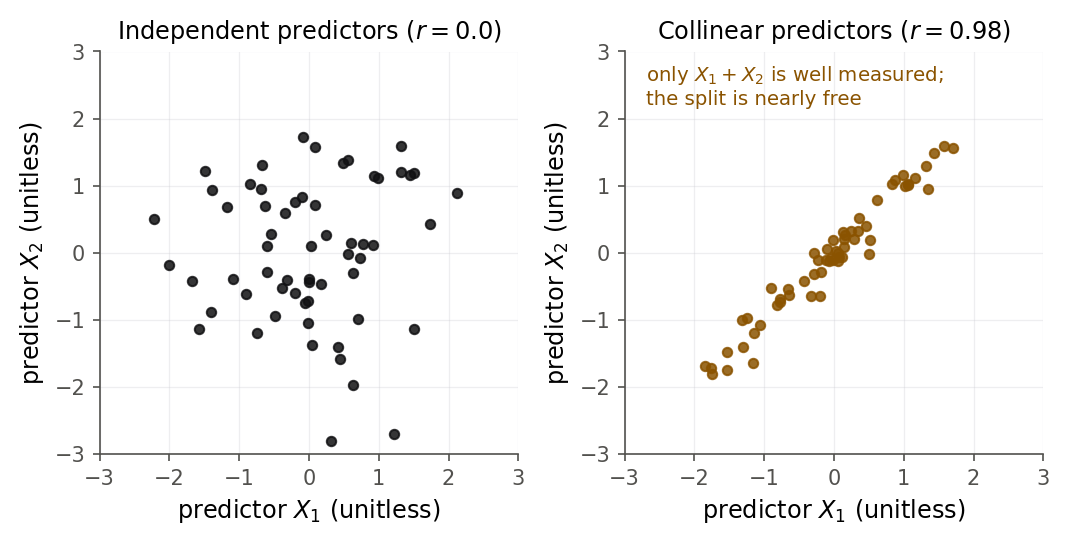
Figure 2:When predictors are independent (left) the data pin down each coefficient. When they are collinear (right) only their sum is well measured; the split into separate coefficients is nearly free to move, which is why collinear coefficients have huge standard errors.
The variance inflation factor (Definition 12.2) measures exactly how much the variance is inflated.
The full model, and why its coefficients misbehave
Fit the full model first, so the symptoms are concrete. The response is brozek, percent
body fat by Brozek’s formula, and the thirteen predictors are the tape and scale
measurements. Recall from 4.2 Correlation and the regression slope that for a single predictor, is just the
squared correlation; with many predictors keeps climbing as you add columns, whether or
not they help, so a high alone proves nothing.
You saw a small version of this in 8.5 Added-variable plots, where a twenty-man body-fat table had a triceps and a thigh measurement so correlated that their coefficients turned unstable. Here the same disease appears at full scale, with thirteen tangled predictors instead of two. A quick look at the correlations among the size measurements confirms the diagnosis.
round(cor(fat[, c("weight", "chest", "abdom", "hip", "thigh")]), 3) weight chest abdom hip thigh
weight 1.000 0.894 0.888 0.941 0.869
chest 0.894 1.000 0.916 0.829 0.730
abdom 0.888 0.916 1.000 0.874 0.767
hip 0.941 0.829 0.874 1.000 0.896
thigh 0.869 0.730 0.767 0.896 1.000print(fat[["weight", "chest", "abdom", "hip", "thigh"]].corr().round(3)) weight chest abdom hip thigh
weight 1.000 0.894 0.888 0.941 0.869
chest 0.894 1.000 0.916 0.829 0.730
abdom 0.888 0.916 1.000 0.874 0.767
hip 0.941 0.829 0.874 1.000 0.896
thigh 0.869 0.730 0.767 0.896 1.000Every pair correlates above 0.7, and weight with hip reaches 0.941. These columns are near-duplicates of one another.
Formula
In words: regress predictor on the remaining predictors, see how well they predict it, and is one over the leftover fraction. If is unrelated to the others, and . If the others explain 90 percent of it, and . A common rule of thumb flags (equivalently ) as serious, though the cutoff is a convention, not a law.
The shape of that formula is worth a look, because it explains why a little collinearity is harmless and a lot is a disaster. Figure 3 plots the VIF against . The curve is nearly flat while a predictor is mostly its own, then bends sharply upward as the others close in on reproducing it. Weight, which the other twelve measurements explain 97 percent of, sits far up the steep part.
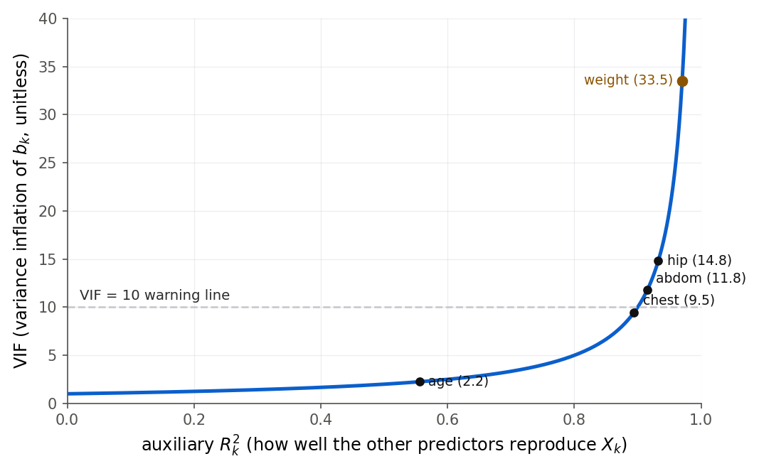
Figure 3:Because the VIF is one over the leftover fraction , it barely moves while a predictor keeps most of its own information, then explodes once the other predictors nearly reproduce it. That steepness is why weight, 97 percent explained by the rest, lands all the way up at VIF 33.5.
The name is literal. The VIF is the factor by which the variance of is multiplied, compared with the variance it would have if were uncorrelated with the other predictors:
In words: the variance of a coefficient is the usual (small when the predictor is spread wide) times the inflation factor. Collinearity enters only through that last factor.
Derivation (the VIF from the auxiliary regression)
Proof. Fix a predictor . By the added-variable construction of 8.5 Added-variable plots, the least-squares coefficient equals the slope from a simple regression of on the part of that the other predictors do not explain. Make that part concrete: run the auxiliary regression of on all the other predictors, and call its residuals . These residuals are with the other predictors’ information removed.
The added-variable result says , a simple-regression slope with the as the predictor. From 2.5 Sampling behavior and the Gauss-Markov theorem, a simple-regression slope with weights has variance . So
Now identify the denominator. The auxiliary regression has total sum of squares and error sum of squares . By the definition of applied to that auxiliary regression,
Substitute:
The first factor is what the variance would be if were free of the others (). The second factor is the price of collinearity. When the other predictors nearly reproduce , and the variance explodes.
R and Python
R’s car package computes every VIF at once. The formula above lets you check any one of
them by hand from a single auxiliary regression.
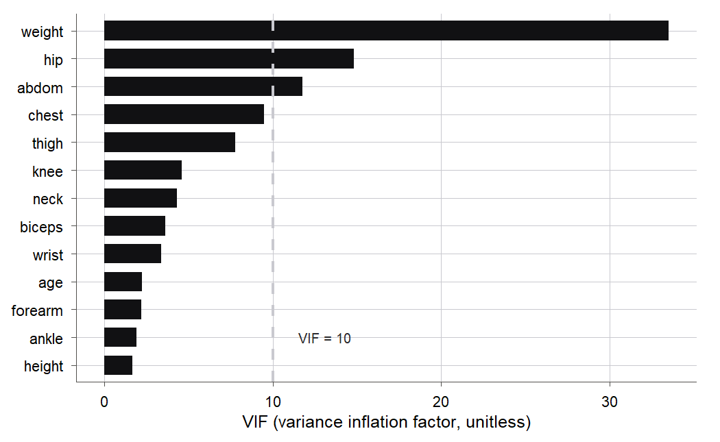
Figure 4:Variance inflation factors, sorted. Weight, hip, and abdomen exceed the usual VIF = 10 warning line, so their individual coefficients are the least trustworthy in the model.
Remedies
There are four honest responses to high VIFs. First, do nothing, if you only care about prediction inside the range of the data: collinearity does not bias or widen its interval much, so a predictive model can carry redundant predictors safely. Second, drop predictors: if weight, hip, and abdomen say nearly the same thing, keep the one you can measure best and discard the rest. Third, combine them into a single index (an average, or a principal component) that captures the shared size signal. Fourth, shrink the coefficients with ridge regression (Section 12.5), which tolerates collinearity by design. What you must not do is read a collinear coefficient as a real causal effect and act on its sign.
Reading about inflated variance is one thing; here is the same disease with a dial on it, so you can decide for yourself how much correlation is too much.
What to notice: as the correlation rises, SE(b1) and the VIF explode together while the SSE of the fit does not move at all, because the data still pin down the sum of the two effects and not the split. Try setting the correlation to 0.99 and then naming a value of b1 the data can rule out. The formula behind the two curves is Definition 12.2 in 12.1 Multicollinearity and the variance inflation factor.
12.2 Choosing among models: selection criteria
Intuition
The full model has redundant predictors; a smaller model might predict just as well and be easier to trust. But which smaller model? With thirteen predictors there are possible subsets. We need a score that ranks them. The obvious score, , is useless for this, because never decreases when you add a predictor: the biggest model always wins, even if the added predictors are noise. Recall from 4.2 Correlation and the regression slope that is squared correlation, a measure of fit, not of prediction. A good selection criterion must instead reward fit while charging a penalty for each extra parameter, so that a predictor earns its place only if it pays for itself.
Four criteria do this, each in its own currency. Adjusted discounts by the degrees of freedom spent. Mallows estimates the total prediction error and compares it to the number of parameters. AIC and BIC trade goodness of fit against a size penalty from information theory. PRESS predicts each case from a model fit without it. They usually agree on the broad message (drop the deadweight) while disagreeing on the exact size, which is itself a lesson: there is no single correct model.
Formula
Let a candidate model have parameters (predictors plus intercept), error sum of squares , and . Let be the mean square error of the largest (full) model, our best estimate of the noise variance . The four criteria are
(adjusted ): like but with and divided by their degrees of freedom. Adding a useless predictor lowers it. Bigger is better.
(Mallows): small is better; a model with no bias has , so you look for models with low that also sit near the line .
, : fit term plus penalty; smaller is better. BIC’s penalty is heavier than AIC’s whenever , so BIC prefers smaller models.
That last claim is easy to see in a picture. Figure 6 draws the two size penalties as straight lines. With men, BIC charges about for each extra parameter while AIC charges only 2, so the BIC line climbs almost three times as steeply. A predictor has to improve the fit more to pay off its heavier BIC toll, which is exactly why BIC lands on smaller models.
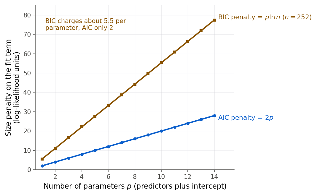
Figure 6:Both criteria charge for size, but with the BIC charges about 5.5 per extra parameter against AIC’s flat 2. The steeper line means each predictor must improve the fit more to earn its place, so BIC settles on leaner models.
The fifth criterion, PRESS, gets its own subsection because it measures something different: honest out-of-sample error.
where is the prediction for case from the model refit with case removed. In words: hide each observation, predict it from the rest, and add up the squared misses. Smaller is better, and unlike , PRESS cannot be driven down just by adding predictors, because a junk predictor helps the fit but hurts the left-out prediction.
Derivation (Mallows )
Proof. We want a criterion that is small when a model’s fitted values are close to the true means , across all cases. Define the target
the total mean squared error of the fitted values, standardized by . Split each term into variance and squared bias with the identity applied to :
For the variance term, the fitted values are with the candidate model’s hat matrix , and , using from 7.3 The hat matrix. So
Now connect to something we can compute, the expected error sum of squares. Write and . Then
because has -th entry so its squared length is , and is idempotent with trace (again 7.3 The hat matrix). Solve for the bias: . Substitute into :
Replace the unknown by the observed and the unknown by the full model’s , and you have Mallows’ statistic:
Two consequences fall out. If the candidate model has no bias (, meaning it contains all the predictors that matter), then and . So unbiased models have : you look for models where is both small and close to . A model that omits an important predictor has , which pushes well above .
R and Python
R’s leaps package searches all 213 subsets and reports the best model of each size.
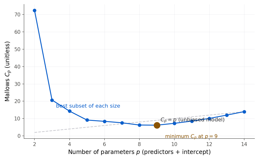
Figure 7:Mallows for the best subset of each size. It drops toward the dashed line and reaches its minimum at eight predictors, the size the criterion prefers. Beyond that, adding predictors raises .
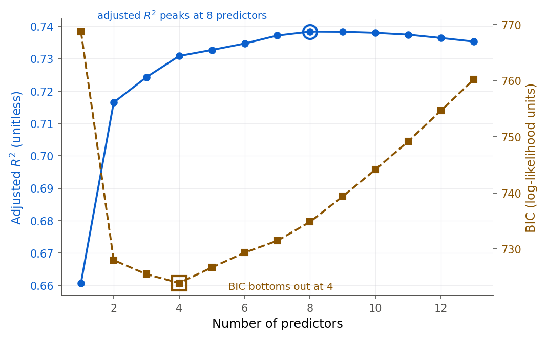
Figure 8:Two criteria, two answers. Adjusted peaks at eight predictors while BIC, penalizing size more heavily, prefers four. Neither is wrong; the honest report is a range of defensible models, not one winner.
Deriving and checking PRESS
PRESS looks expensive: refitting the model times, once per deleted case, is 252 fits per model here. A beautiful identity makes it free. You can get every deleted prediction from a single fit of the full data, using the ordinary residual and the leverage value.
Proof. Write the design matrix with -th row , the full-data estimate , the fitted value , the residual , and the leverage value from 7.3 The hat matrix (the diagonal of the hat matrix). Let be the estimate from the data with case removed, and the deleted prediction. We show
Deleting case changes the cross-product matrix and vector to and . The Sherman-Morrison inverse-update identity (derived and checked in 9.3 Influence: which points actually change the fit) gives
Write , so that and . Multiply the updated inverse by :
where the numerator collapsed to . Now form the deleted prediction:
So each deleted residual is just the ordinary residual divided by , and
High-leverage points (large ) get their residuals magnified, which is right: those are the cases the model props itself up on, and it predicts them worst when they are removed.
Before you accept any one criterion’s verdict, walk the whole ladder of model sizes yourself and watch the four scores pull in different directions.
What to notice: climbs at every single step, so it would always hand you the full model, while adjusted and turn over at eight predictors and BIC turns over at four. Try stopping where each criterion tells you to stop, and read how much each stopping point gives up. The four formulas are in 12.2 Choosing among models: selection criteria.
12.3 The dangers of automatic selection
Intuition
It is tempting to automate the search: let the computer add and drop predictors by their -values until nothing improves. This is stepwise selection (Definition 12.7), and it is available in one line in every statistics package. It is also the source of more bad science than almost any other routine procedure, and you should understand exactly why before you ever use it.
Two things go wrong. The first is overfitting (Definition 12.8): a procedure that chases the best fit on your sample will seize on accidents of that sample, patterns that are noise and will not repeat. The second, subtler and worse, is post-selection inference (Definition 12.9): once you have chosen a model because it fit well, the -values, confidence intervals, and tests that software prints for that model are wrong. They were derived assuming the model was fixed in advance, before you looked at the data. Choosing the model by looking at the data breaks that assumption, and the reported significance becomes fiction.
A demonstration with pure noise
The cleanest way to see the disaster is to run selection on data with no signal at all. Take a response and forty predictors that are all independent random noise, unrelated to the response and to each other. Honest testing should almost never find anything. Selection finds plenty.
set.seed(4210)
noise <- data.frame(y = rnorm(100), matrix(rnorm(100 * 40), 100, 40))
names(noise)[-1] <- paste0("x", 1:40)
pvals <- sapply(1:40, function(j)
  summary(lm(noise$y ~ noise[[paste0("x", j)]]))$coefficients[2, 4])
best5 <- order(pvals)[1:5]
selected <- lm(y ~ ., data = noise[, c("y", paste0("x", best5))])
fstat <- summary(selected)$fstatistic
c(R2 = summary(selected)$r.squared,
  overall_F_pvalue = as.numeric(pf(fstat[1], fstat[2], fstat[3], lower.tail = FALSE)))
R2 overall_F_pvalue
0.13497399 0.01663716We picked the five predictors with the smallest individual -values out of forty pure-noise columns, fit a model on just those five, and got an overall -test -value of 0.017. By the usual rule, that model is “significant at the 0.05 level,” and its looks respectable. Every bit of it is an illusion: there is no relationship in the data at all. The selection step manufactured the significance by cherry-picking, and the test, blind to the cherry-picking, reported it as real.
This is not a one-off fluke of the seed. Figure 10 repeats the whole experiment 2000 times. Under honest testing the overall -value should be uniform on , so only 5 percent should fall below 0.05. After selection, 94 percent do.
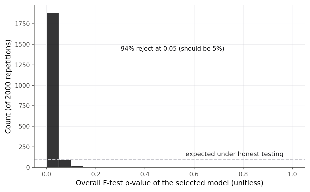
Figure 10:Selecting the five best of forty pure-noise predictors, 2000 times. Honest testing would give a flat histogram with 5 percent below 0.05; instead 94 percent of the selected models look significant. The p-values printed after selection are not trustworthy.
What to do instead
None of this means variable selection is forbidden. It means three things. First, prefer the criterion-based methods of Section 12.2 (compare whole models by , BIC, or cross-validated error) over -value-driven stepwise search, and report that you searched. Second, never quote the -values from a selected model as if the model had been fixed in advance; recall from 8.4 The general linear test that the test’s distribution assumes the comparison was chosen before seeing the data. Third, and most reliably, judge the final model on data it was not chosen with. That is validation, the subject of the next section, and it is the only honest referee for a model you built by searching.
12.4 Validation: train, test, and cross-validate
Intuition
The residuals from a fitted model tell you how well it fits the data it was built on, which is always flattering. To know how well a model predicts, you must test it on data it has never seen. The idea echoes the out-of-sample thinking behind the bootstrap in 5.4 The bootstrap for regression and the prediction intervals of 3.5 Prediction interval for a new observation: honest error estimates come from treating some data as genuinely new.
The simplest version splits the data once: a training set (Definition 12.10) to fit the model, and a test set, held back, to measure its error. The split must be made before any modeling, and the test set must never influence a single choice. A more efficient version, -fold cross-validation (Definition 12.11), splits the data into equal folds, then rotates: each fold takes a turn as the test set while the other folds train the model. Averaging the test errors uses every case for testing exactly once, so it wastes no data. Figure 11 shows the rotation.
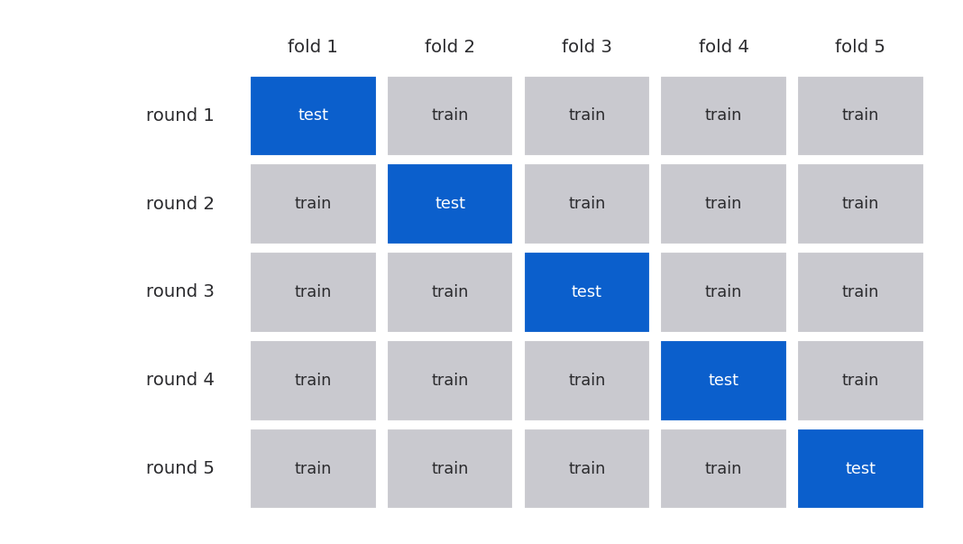
Figure 11:Five-fold cross-validation. The data are split into five folds; each round holds out one fold for testing (orange) and trains on the other four (blue). Every case is tested exactly once, and the five test errors are averaged.
We measure error with the root mean squared error (Definition 12.12), the typical size of a prediction miss, in the units of the response (percentage points of body fat). A smaller one means the model is closer, on average, to the truth for a new man.
The single train/test split
Split the 252 men with a fixed seed so the analysis reproduces, fit on the training set, and compare training error to test error.
-fold cross-validation, written by hand
A single split is noisy: a lucky or unlucky test set can mislead. Cross-validation averages over splits. It is worth writing the loop yourself once, so the mechanism holds no mystery. Assign each case a fold number, then loop: train on the other folds, predict the held-out fold, collect the squared errors.
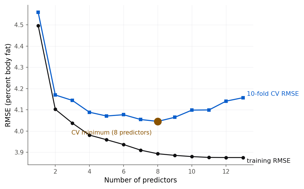
Figure 12:Training error (blue) always falls as predictors are added. Cross-validated error (orange), the honest measure, falls, flattens, and then rises: past a point, extra predictors buy fit on this sample but not accuracy on new men. The gap between the curves is overfitting made visible.
Example 12.5 reported the test RMSE from one split. This widget reruns that split a thousand times, so you can see all the other answers it could just as easily have given you.
What to notice: a single held-out sixty-three men can score this same model anywhere from about 3.0 to 4.9, a spread of nearly two percentage points of body fat. Try five single splits, then a thousand, and watch the mean settle onto the leave-one-out value that the whole dataset already knew. The train, test, and cross-validation definitions are in 12.4 Validation: train, test, and cross-validate.
12.5 A look at shrinkage: ridge and lasso
Intuition
Selection is a blunt instrument: a predictor is either in (full coefficient) or out (zero). Shrinkage (Definition 12.13) offers a gentler alternative. Instead of deleting predictors, it keeps them all but pulls their coefficients toward zero, trading a little bias for a large drop in variance. When predictors are collinear, ordinary least squares can produce enormous coefficients that cancel each other (the negative weight from Example 12.1). Shrinkage refuses to let coefficients grow that large, which stabilizes them.
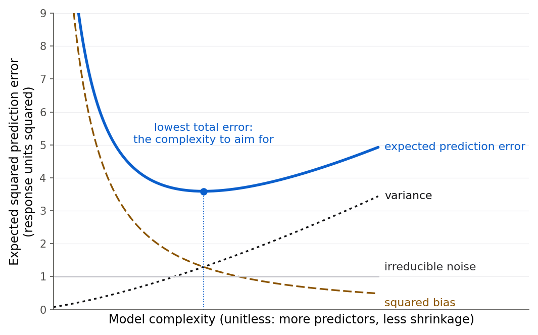
Figure 14:The bias-variance trade-off. As a model grows more flexible, bias falls but variance rises, and expected prediction error is their sum: a U-shape with a sweet spot. Selection and shrinkage are both ways of aiming for that sweet spot instead of the low-bias, high-variance extreme.
Formula
Ordinary least squares minimizes the residual sum of squares. Ridge (Definition 12.14) and lasso (Definition 12.15) add a penalty on the size of the coefficients.
The first term is the usual least-squares loss; it wants a good fit.
The second term is the penalty; it wants small coefficients. The sum runs over the slope coefficients (not the intercept), and predictors are standardized first so the penalty treats them fairly.
is the tuning parameter that sets the strength of the penalty. At both reduce to least squares; as all coefficients are crushed to zero. We choose by cross-validation.
Ridge uses the squared penalty (, the norm); lasso uses the absolute-value penalty (, the norm). The difference sounds minor and is not. Ridge shrinks every coefficient toward zero but rarely to exactly zero. Lasso can set coefficients exactly to zero, so it does variable selection and shrinkage at once. The reason is geometric, shown in Figure 15: the lasso’s constraint region is a diamond with corners on the axes, and the best-fitting contour tends to touch a corner, where a coefficient is zero. Ridge’s constraint region is a smooth disk with no corners.
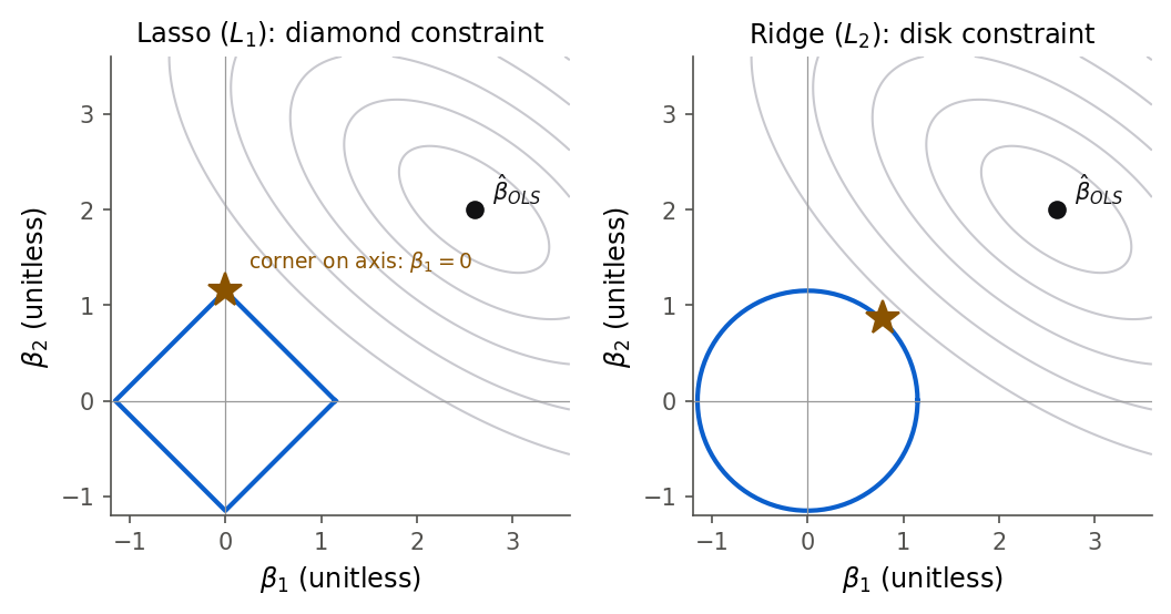
Figure 15:Why lasso zeros coefficients and ridge does not. The solution is where a growing loss contour first meets the constraint region. The lasso diamond has corners on the axes, so contours often meet it at a corner (a coefficient set to zero); the smooth ridge disk has no corners, so it only shrinks.
R and Python
The R package glmnet is the standard tool. Its cv.glmnet fits the whole path of
values and picks one by cross-validation, returning lambda.min (the error minimizer) and
lambda.1se (the largest within one standard error of the minimum, a deliberately
sparser choice). Predictors are standardized automatically.
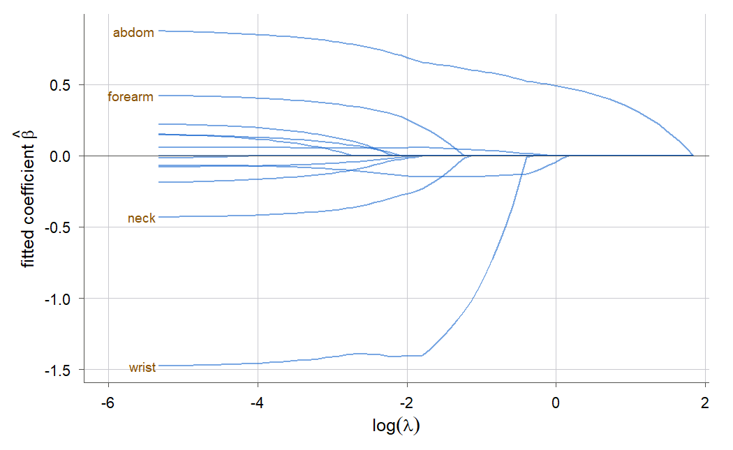
Figure 16:Lasso coefficient paths. As the penalty grows (moving right), coefficients are pulled to exactly zero one after another, so the lasso performs continuous variable selection. Abdomen and wrist are the last to survive.
The plain summary of shrinkage
Ridge and lasso answer the collinearity and selection problems in one move. Ridge keeps every predictor but shrinks the coefficients so no two collinear predictors can blow up against each other; it is the natural tool when you believe many predictors each contribute a little. Lasso shrinks and selects at once, zeroing the coefficients it does not need, so it is the natural tool when you believe only a few predictors matter and you want the model to find them. Both replace the discrete, unstable question “which predictors are in?” with a smooth, tunable dial , set by cross-validation. That is why shrinkage, not stepwise selection, is the modern default when prediction is the goal.
12.6 Chapter summary
You can now handle a regression with more predictors than you can trust. You diagnosed multicollinearity with the variance inflation factor and derived it from an auxiliary regression; you compared candidate models with adjusted , Mallows , AIC, BIC, and PRESS, deriving and proving the deleted-residual shortcut that makes leave-one-out free; you saw, in a pure-noise demonstration, why stepwise selection overfits and why post-selection -values lie; you wrote a -fold cross-validation loop by hand and used a held-out test set to judge a model honestly; and you described and ran ridge and lasso, reading shrinkage as a bias-variance trade made by a tunable penalty. On the body-fat data the eight-predictor candidate beat the full model on every honest measure: lower , lower PRESS, and lower cross-validated error.
Figure 17 puts the whole chapter on one page: diagnose the redundancy, let your goal decide the remedy, choose a model by a prediction-minded score, and confirm the winner on data it never saw.
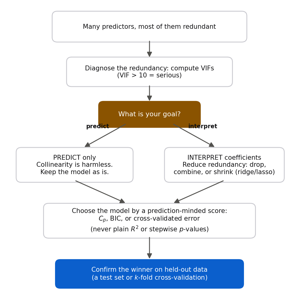
Figure 17:The chapter in one picture. Diagnose the redundancy, let your goal (predict versus interpret) pick the remedy, choose the model by a prediction-minded score, and confirm it on data it never saw.
Key results at a glance
| Result | Statement or formula | Valid when |
|---|---|---|
| Coefficient variance (Theorem 12.4) | general linear model, uncorrelated equal-variance errors | |
| Variance inflation factor (Definition 12.2) | , with the auxiliary | any multiple regression |
| Adjusted | ; bigger is better | comparing models of different size |
| Mallows (Theorem 12.5) | ; unbiased model has | from a near-unbiased full model |
| AIC / BIC | ; smaller is better | compared within one program |
| PRESS shortcut (Theorem 12.6) | least-squares linear fit | |
| CV RMSE | ; smaller is better | folds disjoint, tested once each |
| Ridge / lasso | $\min \mathrm{RSS} + \lambda\sum {\beta_k^2,\ | \beta_k |
Key terms. Multicollinearity, variance inflation factor, auxiliary regression, adjusted , Mallows , AIC, BIC, PRESS, deleted residual, stepwise selection, overfitting, post-selection inference, training and test sets, -fold cross-validation, root mean squared error, bias-variance trade-off, shrinkage, ridge regression, lasso, tuning parameter .
You should now be able to
Diagnose multicollinearity with the VIF and derive it from an auxiliary regression (Theorem 12.4).
Explain what multicollinearity does and does not harm, and list the standard remedies.
Compute and compare adjusted , Mallows , AIC, BIC, and PRESS.
Derive Mallows (Theorem 12.5) and prove the PRESS deleted-residual shortcut (Theorem 12.6).
Explain, bluntly, why stepwise selection and post-selection inference mislead.
Implement -fold cross-validation by hand in R and Python.
Describe ridge and lasso shrinkage and demonstrate them on the body-fat data.
Where this fits. This chapter is the FIT and CHECK stages of The modeling workflow done together and repeatedly: you fit many models, check each for collinearity and prediction error, and iterate toward one you can defend. Chapters 8 through 11 gave you a single multiple regression and the tools to interpret and diagnose it; this chapter faced the harder situation of many competing models and taught you to choose among them by prediction rather than fit. The validation mindset carries straight into 13. Logistic regression, where the same held-out thinking becomes the classification metrics (accuracy, ROC) that judge a logistic model, and the shrinkage and criterion ideas reappear wherever a model has more parameters than the data can comfortably support.
12.7 Frequently asked questions
Q1. Does multicollinearity bias my coefficients? No. Least squares stays unbiased under collinearity: on average the coefficients are still correct. What collinearity does is inflate their variance, so any single sample’s estimates can be wildly off, with flipped signs and huge standard errors. The average is fine; the individual estimate is unreliable.
Q2. If collinearity does not hurt prediction, why care about it? It depends on your goal. If you only want to predict body fat for men like those in the data, a collinear model predicts fine and you can ignore the VIFs. If you want to interpret coefficients (to say which measurement matters and by how much), collinearity makes those coefficients meaningless, and you must fix it by dropping, combining, or shrinking predictors.
Q3. Which selection criterion should I use? For interpretation, BIC and its heavier penalty give you a lean, defensible model. For prediction, cross-validated error is the most direct answer, and Mallows is a fast, well-motivated stand-in. Do not agonize over small differences: report that the criteria pointed to a range of models (here, four to eight predictors) and pick within that range for a reason you can state.
Q4. Why is the of the full model always equal to the number of its parameters? By construction. , and for the full model , so and $C_p = (n - p_{\text{full}})
(n - 2p_{\text{full}}) = p_{\text{full}}C_pC_p = p$ line.
Q5. Is a lower PRESS always better? As a comparison of models on the same data, yes: lower PRESS means better leave-one-out prediction. But PRESS is still an in-sample estimate in the sense that it uses the same 252 men to build and to test (just never the same man for both at once), so it can be optimistic if the whole dataset is unusual. A truly held-out test set, or -fold cross-validation repeated with different seeds, is a stronger check.
Q6. Can I just trust the model my software’s step() function returns? No. Stepwise
selection overfits and its reported -values are invalid (Section 12.3). If you use it,
treat its output as a candidate to be validated on held-out data, never as a finished model,
and never quote its coefficients’ significance as if the model had been chosen in advance.
Q7. Lasso and stepwise both drop predictors. What is the difference? Stepwise makes hard, unstable in-or-out decisions by -value and reports dishonest inference. Lasso makes the decision continuously through a single penalty chosen by cross-validation, shrinking coefficients smoothly and turning them off only as the penalty grows. Lasso is more stable, has a coherent bias-variance justification, and is built for prediction. When in doubt, prefer it.
Q8. Why standardize predictors before ridge or lasso? The penalty or
adds up coefficients measured in each predictor’s own units. Without
standardizing, a predictor measured in small units (and so carrying a large coefficient) would
be penalized more than an identical predictor in large units. Standardizing puts every
predictor on the same scale so the penalty is fair. Both glmnet and the scaled scikit-learn
fit here do this.
12.8 Practice problems
(A) In one sentence each, say what multicollinearity does to the bias of , to the variance of , and to predictions made inside the data range. Then name two of the standard remedies for a predictor with a high VIF.
(A) A predictor has . What is the auxiliary , and how many times larger is than it would be if the predictor were uncorrelated with the others?
(A) Explain why cannot be used to choose between a model with 5 predictors and one with 8 predictors, but adjusted can.
(A) State the rule of thumb that connects a “good” model’s to its number of parameters , and say what a far above indicates.
(A) Why does BIC tend to select smaller models than AIC? Point to the specific term that differs.
(A) In plain words, what does the PRESS statistic measure that ordinary does not?
(A) A student selects predictors by stepwise regression, then reports the model’s -values as evidence it is correct. Name the fallacy and explain it in two sentences.
(A) Describe the difference between what ridge and lasso do to a coefficient, and say which one performs variable selection.
(A) A model’s training RMSE is 3.5 and its 10-fold CV RMSE is 4.6. What does the gap tell you, and which number estimates performance on new data?
(A) Explain why predictors are standardized before applying a ridge or lasso penalty.
(B) Derive (Theorem 12.4) starting from the added-variable fact that is the slope of on the residuals of regressed on the other predictors. Identify where appears.
(B) Show that the auxiliary regression’s error sum of squares equals , and use it to explain why a predictor nearly determined by the others has a nearly zero denominator in its coefficient variance.
(B) Derive Mallows (Theorem 12.5) from the standardized total mean squared error , including the steps and . Conclude that an unbiased model has .
(B) Prove the PRESS deleted-residual shortcut (Theorem 12.6), stating clearly where the Sherman-Morrison inverse update is used.
(B) Show that for the full model, equals its number of parameters exactly. (Start from the definition of and the fact that is the full model’s MSE.)
(B) A high-leverage case has and ordinary residual . Compute its deleted residual, and explain why leave-one-out prediction magnifies the residuals of high-leverage cases.
(B) Explain, using the bias-variance decomposition of prediction error, why a model can have both lower training error and higher test error than a smaller model. Which term of the decomposition rises as the model grows?
(B) Show that as the ridge coefficient of a single standardized predictor tends to zero, and that at it equals the least-squares slope. (Use the one-predictor ridge solution, which you may derive in Problem 19.)
(B) Derive the one-predictor ridge estimator in Problem 18 by setting the derivative of to zero, and interpret the denominator as “signal plus penalty.”
(C) Fit the full model and reproduce the VIFs. Identify every predictor with $\mathrm{VIF}
10$ and, for one of them, confirm the VIF by running its auxiliary regression by hand.
(C) Run the exhaustive best-subset search (R
leaps, or the Python loop) and report the best model of each size with its . State the sizes chosen by , adjusted , and BIC.(C) For the four-predictor best subset (weight, abdomen, forearm, wrist), compute , AIC, BIC, and PRESS. Compare each to the eight-predictor candidate and say which model you would report and why.
(C) Write a function that computes PRESS from a fitted model using the shortcut, and verify it against a brute-force leave-one-out loop on the candidate model. Report both values.
(C) Reproduce the pure-noise post-selection demonstration with a different seed. Report the selected model’s and overall -value, and explain why they are misleading.
(C) Perform a seeded 70/30 train/test split. Fit the full and candidate models on the training set and report both test-set RMSEs. Which model predicts better, and does the order match the training-set fit?
(C) Write a 5-fold cross-validation loop by hand and compare the full model, the eight-predictor candidate, and the four-predictor model (weight, abdomen, forearm, wrist) by CV RMSE. Rank them.
(C) Fit a lasso with
cv.glmnet(R) orLassoCV(Python) to the whole dataset. Report which predictors have nonzero coefficients at the cross-validated penalty, and compare that set to the eight-predictor model.(C) Fit ridge regression across a grid of values and plot the coefficient of
weightagainst . Describe how the coefficient changes, and connect its behavior to the VIF of 33.5 you found forweight.(C) Using the candidate model, plot the deleted residuals against the ordinary residuals . Which cases move the most, and what property of those cases explains it?
(C) Take the 25 percent of men with the largest leverages and refit the candidate model without them. Report how much the coefficients and PRESS change, and discuss whether the model is being propped up by a few cases.
12.9 Exam practice
These five questions are written in the style of the course exams: each asks you to
explain your reasoning in full sentences, not just to produce a number. Where output is
shown, it was produced on the course machine from fat.csv; read the numbers you need off the
printout and say which you used. Work each one before opening its model answer.
EP 12.1 (concepts, evaluate a claim). The full body-fat model of Example 12.1 was refit and
the weight coefficient and three variance inflation factors were printed.
full <- lm(brozek ~ age + weight + height + neck + chest + abdom + hip +
             thigh + knee + ankle + biceps + forearm + wrist, data = fat)
round(coef(summary(full))["weight", ], 4)
round(car::vif(full)[c("weight", "hip", "abdom")], 2)
Estimate Std. Error t value Pr(>|t|)
-0.0803 0.0496 -1.6198 0.1066
weight hip abdom
33.51 14.80 11.77A student reads the negative weight coefficient and concludes: “holding the other twelve
measurements fixed, heavier men have less body fat, so we should tell clients that gaining
weight lowers their body fat percentage.” Evaluate this claim. Use the variance inflation
factor in your answer, and state clearly what the coefficient can and cannot support.
Model answer
The coefficient is a partial slope: it is meant to describe what happens to body fat when
weight rises by one pound while all other measurements are held fixed. The claim fails
because the data barely contain that comparison. Weight has , which means
the other twelve measurements explain of weight, so men almost
never differ in weight while their chest, abdomen, hip, and thigh stay fixed. The estimate
therefore rests on almost no real contrast: its standard error is inflated by
times, the statistic is only -1.62 with , and the
coefficient is not distinguishable from zero. Multicollinearity inflates the variance of a
coefficient without biasing it, so the negative sign here is an artifact of the near-duplicate
size predictors, not evidence that gaining weight reduces fat. The coefficient cannot support
any advice about changing weight; the honest statement is that this model cannot separate the
effect of weight from the other girths. A weak answer stops at “it is not significant” or
“weight does not matter” without invoking the VIF and the missing contrast, or worse, treats
the negative sign as a real effect to be explained.
EP 12.2 (interpret output in context). An exhaustive best-subset search was run on a
six-predictor version of the model, brozek ~ age + weight + height + abdom + hip + thigh,
reporting the best subset of each size.
rs <- regsubsets(brozek ~ age + weight + height + abdom + hip + thigh,
                 data = fat, nvmax = 6)
ss <- summary(rs)
rbind(Cp = round(ss$cp, 2), adjR2 = round(ss$adjr2, 4), BIC = round(ss$bic, 1))
c(min_Cp = which.min(ss$cp), max_adjR2 = which.max(ss$adjr2), min_BIC = which.min(ss$bic))
[,1] [,2] [,3] [,4] [,5] [,6]
Cp 55.07 6.29 3.88 4.40 5.13 7.00
adjR2 0.6608 0.7165 0.7203 0.7208 0.7212 0.7202
BIC -262.40 -303.10 -302.00 -298.00 -293.70 -288.30
min_Cp max_adjR2 min_BIC
3 5 2The best size-2 model is weight + abdom, the best size-3 model is weight + abdom + thigh,
and the best size-5 model is weight + height + abdom + hip + thigh. Interpret this output.
State which model size each of the three criteria selects, explain in full sentences why
Mallows and BIC land on different sizes, and say which model you would report to a
colleague who wants to interpret the coefficients, with your reason.
Model answer
Mallows is smallest at size 3 (weight + abdom + thigh, ), adjusted
is largest at size 5 (0.72), and BIC is smallest at size 2 (weight + abdom, -303.1). The
criteria disagree because each charges a different price per added parameter. Adjusted
penalizes size only lightly, so it tolerates the largest model that still improves the fit at
all; BIC charges , about 5.5 per parameter with , the heaviest toll, so it
settles on the leanest model; sits between them. All three agree on the substance:
abdomen and weight together capture nearly all the signal ( falls from 55 to 6.3 as
soon as both are in), and height buys essentially nothing for its parameter. For a colleague
who wants to interpret coefficients I would report the BIC or model (two or three
predictors), because a lean model gives coefficients you can actually read and trust, and I
would state plainly that the criteria point to a small range of defensible sizes (two to
three), not a single winner. A weak answer just reads the three minima off the printout without
explaining that the differing penalties per parameter are what drive the disagreement, or
declares one criterion the “correct” one.
EP 12.3 (what would change if). For the four-predictor model
brozek ~ weight + abdom + forearm + wrist, the error sum of squares is
with and parameters. The full model’s estimate of
the noise variance is .
cand4 <- lm(brozek ~ weight + abdom + forearm + wrist, data = fat)
c(SSE = sum(resid(cand4)^2), sigma2_full = summary(full)$sigma^2)
SSE sigma2_full
3994.311 15.904First compute for this model. Then answer: what would change if you estimated not from the full model but from the abdomen-only model, whose residual mean square is 20.38? Compute the resulting and explain, in full sentences, why becomes meaningless with that choice.
Model answer
With the full-model variance, , a little above , which hints at slight bias in this small model. If instead is estimated from the abdomen-only model, that estimate is 20.38, and , a negative and nonsensical value. The reason is that the abdomen-only model is underspecified: it has left real predictive signal in its residuals, so its residual mean square estimates plus a positive bias, not itself, and it comes out too large. The derivation of assumes is unbiased for the true , which is exactly why you take it from the full model (or a large near-unbiased model), whose residual mean square is unbiased. A biased, inflated shrinks every term, pushes all values far below , and destroys both the “” benchmark and any honest comparison between models. A weak answer computes -46.0 but does not explain that the abdomen-only mean square is biased upward because it omits real predictors, nor connects the failure to the unbiasedness assumption behind .
EP 12.4 (evaluate a claim, interpret output). Three models were compared by their training RMSE and by 5-fold cross-validated RMSE on the full body-fat data: the thirteen-predictor full model, the eight-predictor candidate (age, weight, neck, abdomen, hip, thigh, forearm, wrist), and a two-predictor model (abdomen, weight).
set.seed(4210)
folds <- sample(rep(1:5, length.out = nrow(fat)))
# training RMSE and 5-fold CV RMSE for each model
full train RMSE 3.876 5-fold CV RMSE 4.097
cand8 train RMSE 3.893 5-fold CV RMSE 4.003
two train RMSE 4.103 5-fold CV RMSE 4.183A student argues: “the full model has the lowest training RMSE (3.876), so it predicts best; report the full model.” Evaluate this argument. Say which number estimates how the model will do on a new man and why, explain why the ranking flips between the two columns, and state which model you would report.
Model answer
The argument confuses fit with prediction. Training RMSE can only fall or stay equal as predictors are added, because least squares fits the very sample it is scored on, so the full model’s lowest training RMSE is guaranteed by its size and is not evidence of better prediction. The honest measure is the 5-fold cross-validated RMSE, which scores each man with a model that did not train on him. By that measure the eight-predictor candidate is best (4.003) and the full model is the worst of the three (4.097): the five extra predictors in the full model fit training-set noise that does not carry over to new men, so the ranking flips between the columns. The two-predictor model has the highest CV RMSE (4.183), so it underfits: too few predictors hurt as well. I would report the eight-predictor candidate, because it minimizes the out-of-sample error, and I would note that CV RMSE, not training RMSE, is the number that estimates accuracy on a new man. A weak answer says the full model “overfits” without noting that training RMSE must decrease with size, fails to name CV RMSE as the out-of-sample estimate, or overlooks that the two-predictor model underfits.
EP 12.5 (what would change if). A lasso was fit to the whole body-fat data with the penalty
chosen by cross-validation, and the coefficients were read at two penalties,
lambda.min (the error minimizer) and the sparser lambda.1se.
X <- as.matrix(fat[, preds]); Y <- fat$brozek
set.seed(4210)
cvl <- cv.glmnet(X, Y, alpha = 1)
round(cbind(min = coef(cvl, s = "lambda.min")[, 1],
            onese = coef(cvl, s = "lambda.1se")[, 1]), 3)
min onese
(Intercept) -13.683 -6.733
age 0.055 0.052
weight -0.065 0.000
height -0.081 -0.149
neck -0.403 -0.137
chest 0.000 0.000
abdom 0.830 0.635
hip -0.147 0.000
thigh 0.171 0.000
knee 0.000 0.000
ankle 0.086 0.000
biceps 0.114 0.000
forearm 0.387 0.112
wrist -1.437 -1.265At lambda.min eleven predictors have nonzero coefficients; at lambda.1se only six do.
Explain what happens to the coefficients as increases from lambda.min to
lambda.1se, why the lasso sets some coefficients exactly to zero while ridge regression would
not, and what would change if the predictors were not standardized before fitting.
Model answer
As grows from lambda.min to lambda.1se, the penalty on coefficient size gets
heavier, so every coefficient is pulled harder toward zero and five more predictors (weight,
hip, thigh, ankle, biceps) reach exactly zero, leaving six nonzero. The lasso can zero
coefficients because its penalty has corners on the coordinate axes: as
the least-squares loss contour grows outward it tends to first touch the diamond-shaped
constraint region at a corner, where one coefficient is exactly zero, so the lasso performs
variable selection as it shrinks. Ridge regression uses the penalty ,
whose constraint region is a smooth disk with no corners, so it shrinks every coefficient
toward zero but essentially never to exactly zero; ridge would keep all thirteen predictors. If
the predictors were not standardized, the penalty would be unfair, because it sums coefficients
measured in each predictor’s own units: a predictor recorded in small units carries a naturally
large coefficient and would be penalized more heavily, so it would be shrunk and zeroed first
for a reason unrelated to its importance. Standardizing puts every predictor on a common scale
so the penalty compares them fairly, and without it the set of surviving predictors would
change arbitrarily. A weak answer says only that “the coefficients shrink” without the corner
geometry that explains the exact zeros, or cannot say why standardization matters for a fair
penalty across differing units.
Chapter game
Resumen del capítulo (en español)
Este capítulo trata el problema de tener demasiados predictores, casi todos redundantes, usando
datos de grasa corporal de 252 hombres (fat.csv): se predice el porcentaje de grasa, medido por
pesaje bajo el agua, a partir de trece medidas de cinta métrica. Al ajustar el modelo completo,
parece bueno, pero los coeficientes no tienen sentido (el de peso sale negativo).
La causa es la multicolinealidad (multicollinearity): los predictores están muy
correlacionados, así que el modelo no puede repartir el efecto compartido.
El factor de inflación de la varianza (variance inflation factor, VIF), , mide el daño. Lo derivamos de una regresión auxiliar y mostramos que : la colinealidad infla la varianza del coeficiente por ese factor. Para el peso, .
Para elegir entre modelos usamos criterios que premian la predicción, no el ajuste: ajustado, el de Mallows (Mallows’ Cp) (que derivamos, con para un modelo sin sesgo), AIC, BIC y PRESS, cuyo atajo del residuo eliminado, , demostramos. El modelo de ocho predictores elegido tiene y menor PRESS que el modelo completo.
Advertimos sobre los peligros de la selección paso a paso (stepwise selection): sobreajusta, y los valores posteriores a la selección son falsos (una demostración con puro ruido produce modelos “significativos” el 94 por ciento de las veces). La solución honesta es la validación (validation): división en entrenamiento y prueba, y validación cruzada de particiones (k-fold cross-validation), que escribimos a mano. El modelo pequeño predice mejor fuera de la muestra. Finalmente, presentamos la contracción (shrinkage): ridge y lasso encogen los coeficientes hacia cero, equilibrando sesgo y varianza; el lasso además selecciona variables. Es la respuesta moderna cuando el objetivo es predecir.