On the evening of January 27, 1986, engineers at Morton Thiokol and NASA argued on a conference call about whether to launch the space shuttle Challenger the next morning. The forecast for Cape Canaveral was cold, near freezing, colder than any previous launch. The concern was the rubber O-rings that sealed the joints of the solid rocket boosters. In the cold the rubber stiffens, and a stiff O-ring might not seal in time to hold back the burning gas. The engineers had data from 23 earlier flights: for each one, the temperature at launch and the number of O-rings, out of six, that showed heat damage afterward.
Figure 1 shows that data. Damage happened on both warm and cool flights, but the coldest launches carried the worst incidents, and the launch under discussion would be far colder than anything on the record. That is the hard part. Every flight that had ever flown did so at 53 degrees Fahrenheit or warmer. The predicted launch temperature was about 31 degrees, off the left edge of all experience. To say anything about the risk at 31 degrees, you have to extend a pattern past the last data point, which is exactly the move a statistician is trained to distrust.
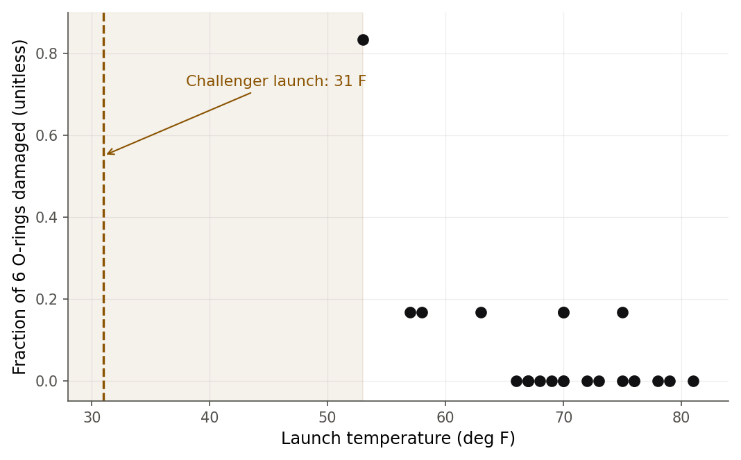
Figure 1:The 23 flights before Challenger. Damage was worst at the coolest launches, and the 31 degree launch decision (dashed line) sat far below every temperature the program had ever flown, so judging its risk means extrapolating.
The response here is not a number like work hours or savings rate. It is closer to a yes-or-no: did an O-ring fail or not. Straight-line regression, the tool of the last eleven chapters, is built for a continuous response and breaks in specific ways when the outcome is binary. This chapter builds the right tool. You will learn the logistic regression model, the odds and log-odds that make it linear, how to fit it by maximum likelihood when no formula gives the estimates, how to read its coefficients as odds ratios without the usual mistakes, how to test them, and how to judge how well the model separates the two outcomes. By the end you will be able to put a number on the risk the Challenger engineers were arguing about, and to say honestly how much to trust it.
13.1 Why a straight line fails, and what to use instead
Intuition
Start with what goes wrong. Suppose you code the response as for a positive outcome (an O-ring damaged, a diabetes test positive) and otherwise, and you fit the ordinary line . Three things break.
First, the fitted line is unbounded. A line keeps rising as grows, so it eventually predicts probabilities above 1 and, going the other way, below 0. Figure 2 shows the least-squares line through the diabetes data sliding straight out of the range where a probability has to live.
Second, the spread is not constant. A response has variance , where is the probability that . That variance is largest near and shrinks toward zero as approaches 0 or 1, the upside-down parabola in Figure 3. A coin near 50-50 is the hardest to call, so its outcome is the most variable; a coin that almost always lands heads is nearly a sure thing, so it barely varies. The spread is fixed by the mean. So the constant-variance assumption behind least squares (2.1 The simple linear regression model) is false by construction, and the weighting that would fix it changes with the mean, an idea we met in weighted least squares (10.4 Weighted least squares).
Third, the errors cannot be normal. If is only ever 0 or 1, then for a given the “error” takes just two values, so the normal error model that justified our and inference simply does not apply.
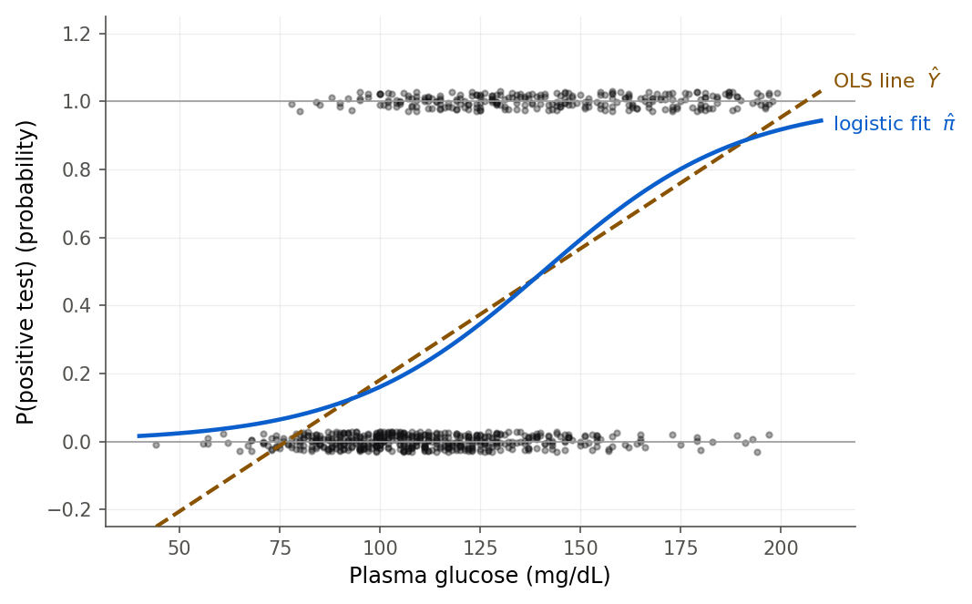
Figure 2:The least-squares line (red dashed) leaves the range a probability must stay in, dropping below 0 and climbing above 1. The logistic curve (blue) bends to fit inside the band.
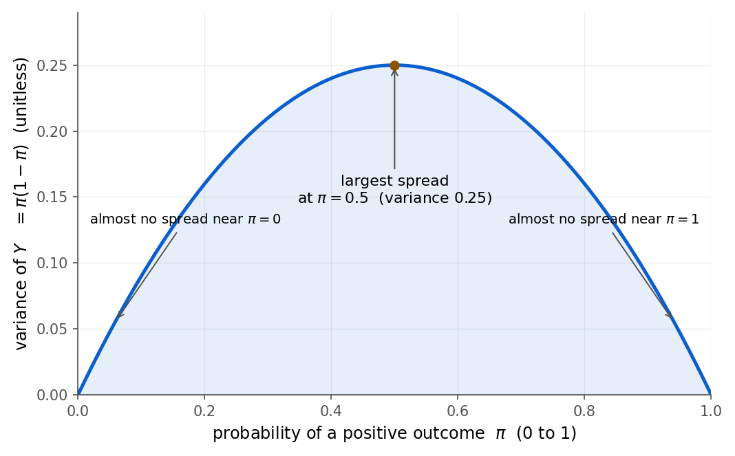
Figure 3:The variance of a yes-or-no outcome is not a free constant: it equals , peaking at and vanishing at both ends. Because the spread is welded to the mean, the constant-variance assumption of least squares cannot hold for a binary response.
The fix is to model the probability directly and to bend the line so it can never leave . The bend is the S-shaped logistic curve in the figure.
From probability to odds to log-odds
The bridge is the odds (Definition 13.1).
A probability of 0.5 is odds of 1 (even money). A probability of 0.75 is odds of 3 (three to one). As climbs toward 1 the odds shoots off to infinity, and as falls toward 0 the odds falls toward 0 but never goes negative. Figure 4 draws this mapping. Odds stretch the bounded probability scale onto the half-line .
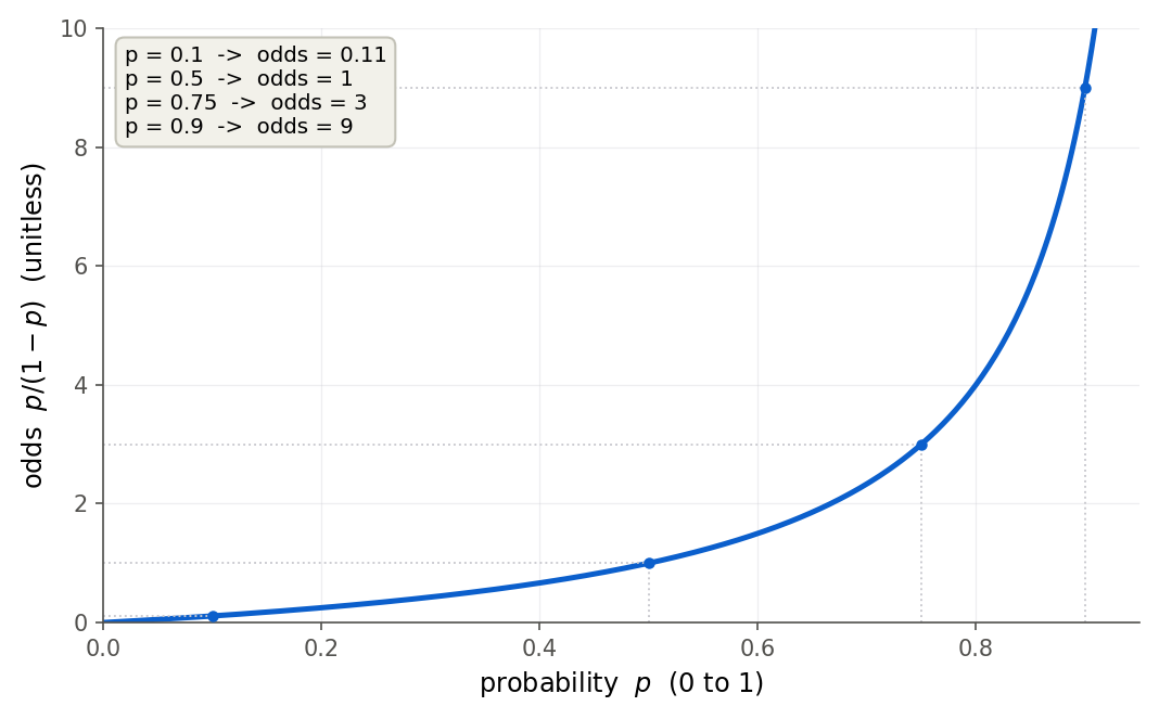
Figure 4:Odds as a function of probability. Equal steps in probability are not equal steps in odds: from 0.5 to 0.75 the odds triples, but from 0.75 to 0.9 it triples again, so the odds scale expands as you approach certainty.
Taking one more step, the log-odds or logit (Definition 13.2) is the natural logarithm of the odds:
In words: the logit is the log of the odds. The logarithm sends onto the whole real line , the same range a linear predictor can take. That is the whole trick. We cannot set a probability equal to a line, because one is bounded and the other is not, but we can set the logit of the probability equal to a line.
The logistic regression model
The logistic regression model (Definition 13.3) for a binary response says the log-odds is linear in the predictors:
where is the probability that case has a positive outcome, the ’s are the regression parameters (with of them counting the intercept), and are the predictors for case . Writing for the linear predictor, we solve the logit equation for to get the model on the probability scale:
In words: the probability is the linear predictor passed through the logistic function , the S-curve of Figure 5. The function is squashed to lie strictly between 0 and 1, so no matter what the coefficients are, the predicted probability is always a legal probability.
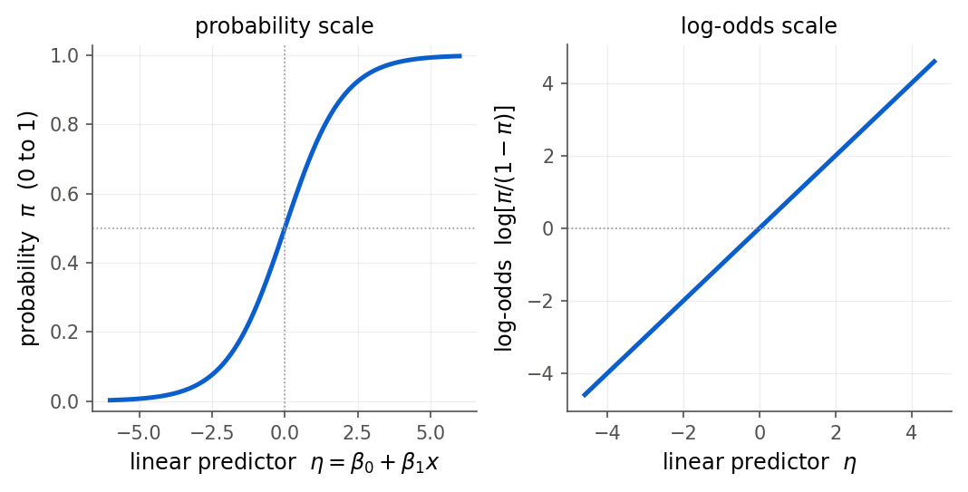
Figure 5:Left: the logistic function turns any linear predictor into a probability between 0 and 1. Right: on the log-odds scale the same relationship is a straight line, which is why logistic regression is a linear model in disguise.
The two links in the term generalized linear model are visible here. There is a random part, being 0 or 1 with probability , and a systematic part, the linear predictor , joined by the link function logit that maps the mean onto the linear scale. Ordinary regression is the same picture with the identity link and a normal response; Chapter 14 makes the family explicit and adds the Poisson member (14.6 One family: the generalized linear model).
R and Python
For the O-ring data the response is grouped: each flight contributes six O-rings, of which
were damaged. That is a binomial count, and logistic regression handles it with the
same machinery, modeling the probability that a single O-ring is damaged at
temperature . In R you pass the two-column response cbind(successes, failures) to
glm with family = binomial; in Python you give statsmodels the two counts on the left of
the formula.
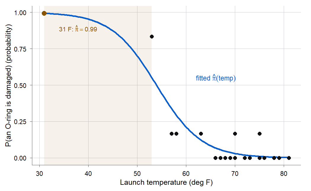
Figure 6:The fitted logistic curve extended to the launch temperature. At 31 degrees (red point, shaded extrapolation region) the model predicts about a 0.99 probability of damage to any given O-ring.
That 0.99 is easier to weigh honestly once you have walked the curve down there yourself.
One slider moves the launch temperature along the fitted curve through the 23 flights. The readouts give the fitted probability, the odds, the expected number of damaged rings out of six, and whether any flight was ever launched that cold.
What to notice. Inside the data the curve is gentle, but the moment you cross 53 degrees into the shaded strip the fitted probability climbs from 0.550 to 0.993 with no observation underneath it. Try this. Park the slider at 31 degrees, read the “none: extrapolating” label, and ask what would have to stay true about the world for that number to hold. Back to Section 13.1.
13.2 Fitting by maximum likelihood
Intuition
In simple regression we had formulas: and . Logistic regression has no such closed form. The reason is the S-curve: the probability is a nonlinear function of the coefficients, so setting derivatives to zero gives equations you cannot solve with algebra. Instead we choose the coefficients that make the observed data most probable, the principle of maximum likelihood we first met for the normal model in Chapter 2, and we find them by climbing the likelihood hill numerically.
The likelihood and log-likelihood
Let case have trials and successes (for a plain binary response and ; for the O-rings ). Given the probabilities , the successes are independent binomial counts, so the likelihood, the probability of the observed data as a function of the coefficients, is
where each depends on through the linear predictor . In words: the likelihood multiplies together, across all cases, the binomial chance of seeing exactly the successes we observed, so larger values point to coefficients the data favor. Taking logs turns the product into a sum, the log-likelihood:
where collects the binomial coefficients , which do not involve and so do not affect where the maximum sits. In words: the log-likelihood rewards coefficients that put high probability on the successes we saw and high non-probability on the failures we saw.
The score equations
Proof. We want the that maximizes , so we differentiate and set the result to zero. Two facts about the logistic link make the algebra collapse. First, from ,
Substituting these into and collecting terms,
Second, differentiate with respect to to get exactly . Using the chain rule with (the -th predictor value for case , with for the intercept),
Setting all partial derivatives to zero gives the score equations. Stacking them with the design matrix (rows ), the fitted mean vector with entries , and the response vector ,
In words: at the maximum-likelihood estimate, each predictor is orthogonal to the residuals , exactly the condition the least-squares normal equations imposed in 7.1 The model and least squares in matrix form. The difference is that here bends through the logistic link, so the equations are nonlinear in and cannot be solved in closed form.
Newton-Raphson and IRLS
Proof. To solve we use Newton’s method, which needs the matrix of second derivatives. Differentiating the score once more, and using ,
so the Hessian is with the diagonal weight matrix . Each weight is the variance of , largest for cases near and small for cases the model is already sure about. A Newton step from a current guess is
with , evaluated at . Now the tidy part. Define the working response . Then
using . Multiplying the Newton step by shows it is equivalent to
That is the formula for a weighted least squares fit of the working response on with weights (10.4 Weighted least squares). Because and change each time updates, we recompute and refit, which is why the method is called iteratively reweighted least squares (IRLS). Starting from any reasonable guess, the iterates climb the concave log-likelihood to its single maximum.
R and Python
The centerpiece is worth doing by hand once, so IRLS stops being a black box inside glm.
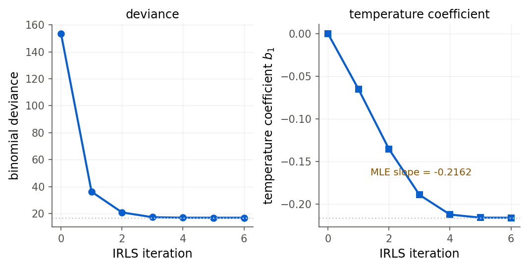
Figure 8:IRLS converges fast. The deviance (left) collapses to its minimum and the temperature coefficient (right) reaches its maximum-likelihood value within about five steps, because the log-likelihood is concave with a single peak.
IRLS climbs the log-likelihood in six passes; climb it by hand once and the algorithm stops being a black box.
Two sliders set and for ten binary observations at ten doses. The log-likelihood readout scores every setting you try, and it is exactly the quantity IRLS is climbing.
What to notice. The log-likelihood is always negative and has a single peak, so every move away from the best setting costs you something, which is the concavity the proof relied on. Try this. Get the log-likelihood as close to zero as you can by hand, then set and watch the S-curve flatten and the odds ratio drop to 1. Back to Section 13.2.
13.3 Reading coefficients as odds ratios
Intuition
A slope in ordinary regression is easy to say out loud: one more unit of adds to the predicted response. The logistic slope is not that, and saying it that way is the single most common mistake in applied logistic regression. The coefficient lives on the log-odds scale, so before interpreting it we have to undo the log.
Here is the wrong reading first, because you will hear it constantly. For the diabetes model below, the glucose coefficient is about 0.04. The tempting sentence is “each extra unit of glucose raises the probability of a positive test by 0.04.” That is wrong twice over. The coefficient is not a change in probability at all, and the effect on probability is not even constant: it depends on where you start on the S-curve, tiny out in the flat tails and largest in the steep middle. What is constant is the effect on the odds. Figure 10 makes the split visible: one fixed step along the curve gives three different probability jumps but always the same odds multiplier.
Formula
Exponentiate the coefficient. Because , raising by one unit changes the log-odds by , so it multiplies the odds by :
The quantity is the odds ratio (Definition 13.6) for a one-unit increase in . In words: a one-unit rise in multiplies the odds of a positive outcome by , whatever the starting odds were. An odds ratio of 1 means no effect; above 1 the odds go up, below 1 they go down. This is the same “logs make it multiplicative” logic as the log-transformed response in 10.2 The log transformation and reading its coefficients, moved onto the odds scale. For a step of units the odds ratio is , which is how you report an effect per 10 units or per decade of age.
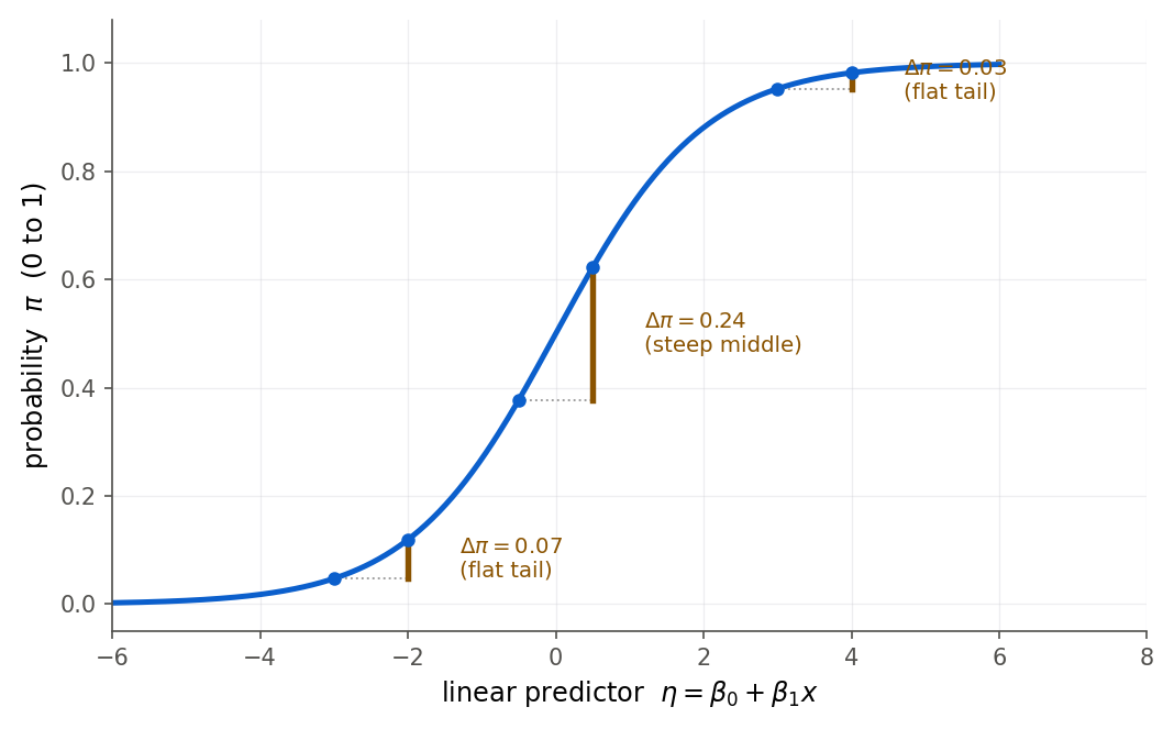
Figure 10:The same one-unit step multiplies the odds by the same fixed factor everywhere (here about 2.72), yet the jump in probability is large in the steep middle and small in the flat tails. That is why the odds ratio is a single honest number but “the change in probability” is not.
R and Python
Figure 11 shows the single-predictor fit. The probability climbs smoothly with glucose, steeply through the middle of the range and flattening at both ends, the S-curve doing its job.
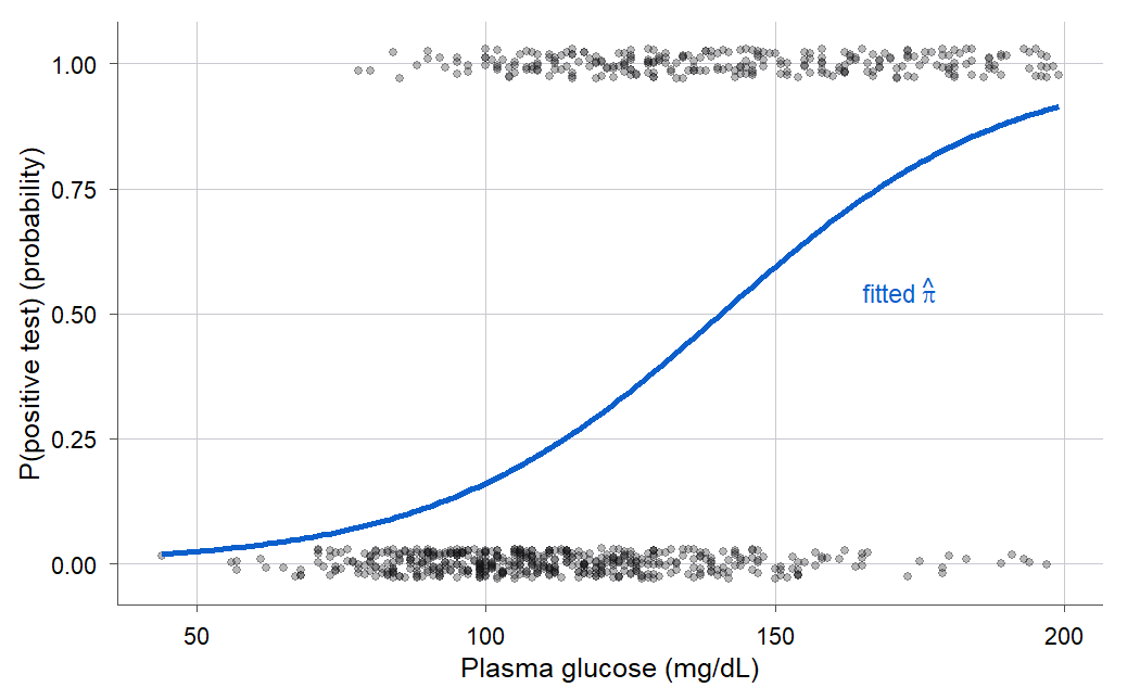
Figure 11:The single-predictor logistic fit to the Pima data. The probability of a positive test rises with glucose, but the heavy overlap of the two outcome bands warns that glucose alone will not cleanly separate positives from negatives.
The split between a constant odds ratio and a moving probability change is worth watching move under your finger.
The curve is the fitted glucose model . One slider sets where the step starts, the other sets its size , and the readouts give both fitted probabilities, their difference, and the odds ratio .
What to notice. Hold at 40 and slide the starting point: the change in probability runs from about 0.12 at glucose 60 up past 0.33 near glucose 100 and back down, while the odds ratio never leaves 5.080. Try this. Hunt for the starting glucose with the largest probability jump, and notice it sits in the steep middle of the S-curve, never in a tail. Back to Section 13.3.
13.4 Testing coefficients: Wald and likelihood-ratio
Intuition
The first section fit the model; the obvious next question is which predictors are pulling their weight. There are two standard tests, and they answer the same question by different routes. The Wald test asks how many standard errors a coefficient sits from zero, using the fitted model alone. The likelihood-ratio test asks how much the fit gets worse when you delete the predictor and refit, comparing two nested models the way the general linear test compared them for ordinary regression (8.4 The general linear test).
Formula
For the Wald test of , the statistic is
In words: the Wald statistic counts how many standard errors the estimate sits from zero, and under the null that distance follows a standard normal curve. Here is the standard error printed by the fit. You can compare to a chi-square with one degree of freedom instead, which gives the same test. The Wald confidence interval for is , and exponentiating its endpoints gives a confidence interval for the odds ratio. These standard errors and the normal reference are large-sample approximations, exact only as . With a small sample or a near-perfect predictor they can mislead.
The likelihood-ratio test uses the deviance (Definition 13.7). For a fitted model with maximized log-likelihood , the deviance is
where is the log-likelihood of the saturated model that fits every observation perfectly (), and are the fitted counts.
In words: the deviance measures how far the fitted model sits from a perfect fit, smaller being better; it is the logistic stand-in for the residual sum of squares. To compare a full model to a nested reduced model that drops predictors, the likelihood-ratio statistic is the increase in deviance,
with the number of coefficients set to zero. The special case comparing the full model to the intercept-only model uses the null deviance as and tests whether any predictor matters at all.
R and Python
Figure 13 plots the odds ratios and their intervals on a log scale, each rescaled to an interpretable step. An interval that clears the vertical line at 1 flags a predictor distinguishable from no effect; age’s interval straddles it.
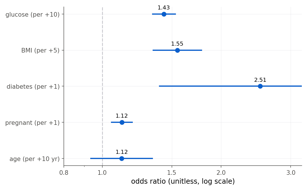
Figure 13:Odds ratios per interpretable step for the Pima model, with Wald 95 percent intervals on a log scale. Every predictor’s interval clears the no-effect line at 1 except age, matching its non-significant test.
The Wald and likelihood-ratio tests usually agree, but not always. The likelihood-ratio test is generally the more reliable of the two, because it uses the actual shape of the log-likelihood rather than a single quadratic approximation at the estimate. In the awkward case of a very large coefficient (a predictor that nearly separates the two outcomes), the Wald standard error can inflate and pull its toward zero, hiding a strong effect. The likelihood-ratio test does not suffer that failure. When the two disagree, trust the likelihood-ratio test. Figure 14 shows the reason in one picture: the Wald test replaces the true log-likelihood with a symmetric parabola matched at the peak, and when the true curve is lopsided the parabola drifts away from it, so the two tests measure different drops down to the null.
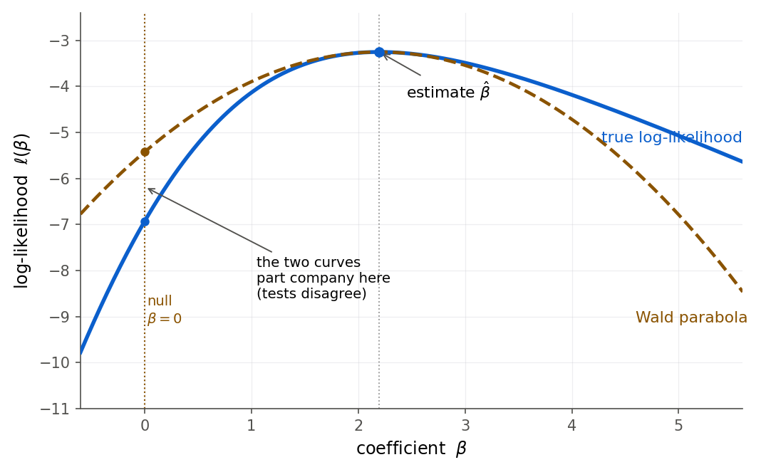
Figure 14:The Wald test judges a coefficient by a symmetric parabola fitted at the peak of the log-likelihood, while the likelihood-ratio test uses the true curve. When the curve is skewed, the two part company away from the peak and can reach the null at different heights, which is why they can disagree and why the likelihood-ratio test is the one to trust.
13.5 How good is the fit? Classification, ROC, and data checks
Intuition
A model can have significant coefficients and still classify poorly, so the last step is to ask how well the fitted probabilities actually separate the two outcomes. We keep this light: a classification table, an ROC curve, and, first, a look at whether the data deserve trust at all.
Data first: the disguised zeros
Recall the impossible zeros from 13.3 Reading coefficients as odds ratios. Figure 15 counts them.
Serum insulin is zero for 374 of 768 women and skinfold thickness for 227; a living person has
neither. These are missing values recorded as zeros, and a model that swallows them whole will
estimate, for instance, a nonsense insulin slope driven by a spike of fake zeros. This is why
we set glucose and BMI zeros to NA before fitting and why we left insulin and triceps out of
the model entirely. The lesson generalizes: look at your predictors before you trust any
coefficient, because the software will fit whatever you feed it.
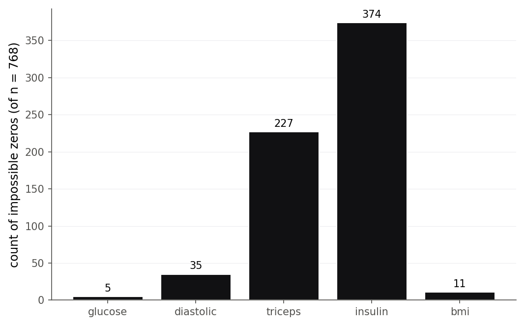
Figure 15:Disguised missing data in the Pima predictors. Insulin and triceps are zero for hundreds of women, which is physiologically impossible, so those zeros are missing values in disguise and must be handled before modeling.
Classification table and ROC
To turn probabilities into yes-or-no predictions, pick a threshold (0.5 is the default) and predict positive when exceeds it. Cross-tabulating predictions against truth gives a classification table, from which sensitivity (the fraction of true positives caught) and specificity (the fraction of true negatives correctly cleared) follow (Definition 13.8). Because one threshold is an arbitrary choice, the ROC curve sweeps every threshold at once, plotting sensitivity against one-minus-specificity; the area under the curve (AUC) summarizes the whole sweep as the probability that the model scores a random positive above a random negative (Definition 13.9).
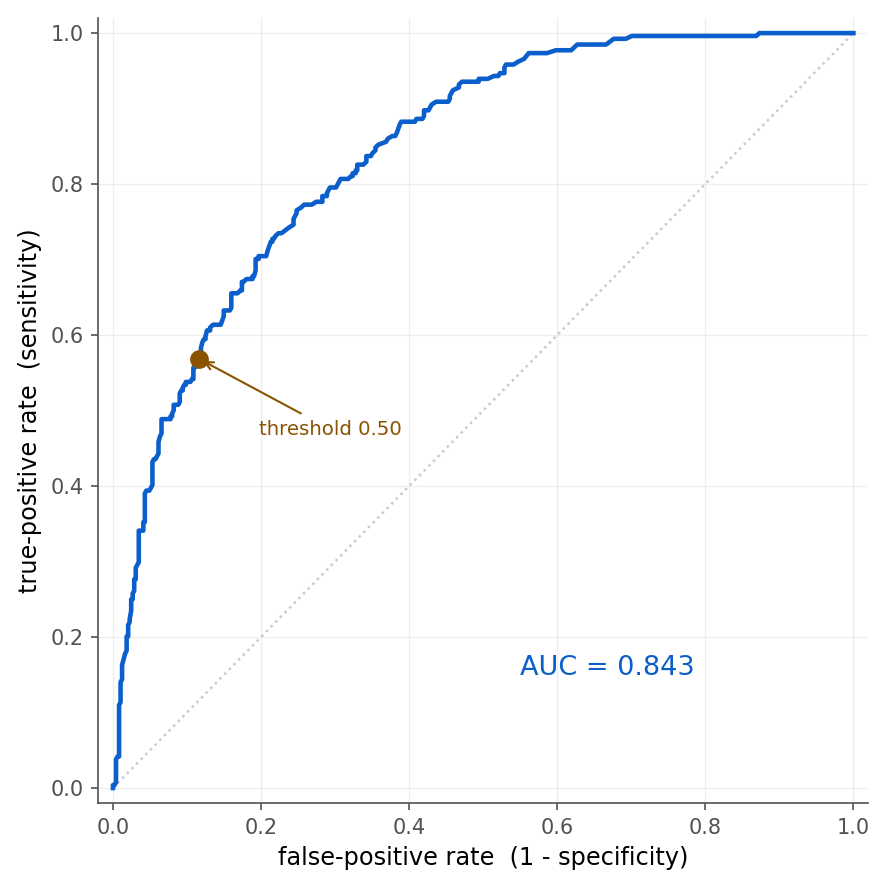
Figure 16:The ROC curve sweeps every classification threshold. The curve bows above the diagonal (chance), with AUC 0.84; the red point is the default 0.5 threshold, showing its high specificity but modest sensitivity.
The 0.5 in that table is a choice you made, not something the model handed you, so the fair thing to do is move it.
The ROC curve of the five-predictor model on all 752 women, with an operating point that follows your threshold. Sensitivity, specificity, accuracy, and the cells of the classification table are recomputed from the 752 fitted probabilities at every step.
What to notice. Dropping the threshold from 0.50 to 0.30 lifts sensitivity from 0.568 to 0.784 and cuts the missed positives from 114 to 57, while false alarms climb from 57 to 140 and accuracy falls. Try this. Find the threshold with the highest accuracy, count how many positive cases it still misses, then decide whether you would ship it as a screening test. Back to Section 13.5.
13.6 Chapter summary
This chapter built a regression model for a binary or binomial response. Ordinary least squares fails for a yes-or-no outcome in three ways (unbounded fits, non-constant variance, non-normal errors), and logistic regression fixes all three by making the log-odds linear. Because the S-curve makes the likelihood equations nonlinear, there is no closed-form estimate: maximum likelihood finds the coefficients, and IRLS computes them by repeated weighted least squares. Each coefficient reads as an odds ratio, tested by the Wald and likelihood-ratio tests, and the fitted probabilities are judged by deviance, a classification table, and an ROC curve, after the data are checked for disguised missing values.
Key results at a glance
| Result | Statement or formula | Valid when |
|---|---|---|
| Odds (Def 13.1) | any probability | |
| Logit (Def 13.2) | ||
| Logistic model (Def 13.3) | , | binary or binomial response, independent cases |
| Score equations (Thm 13.4) | , | at the maximum-likelihood estimate |
| IRLS (Thm 13.5) | each Newton step; log-likelihood is concave | |
| Odds ratio (Def 13.6) | (or per units) | log-odds linear in |
| Deviance (Def 13.7) | fitted model vs saturated model | |
| Wald statistic | large sample | |
| Likelihood-ratio | nested models, large sample | |
| Sensitivity, specificity (Def 13.8) | , | a chosen threshold |
| AUC (Def 13.9) | ranking quality, all thresholds |
Key terms
logistic regression, odds, log-odds (logit), linear predictor, link function, maximum likelihood, likelihood, log-likelihood, score equations, iteratively reweighted least squares (IRLS), working response, odds ratio, Wald test, likelihood-ratio test, deviance, saturated model, classification table, sensitivity, specificity, ROC curve, area under the curve (AUC).
You should now be able to
Explain why ordinary least squares is the wrong model for a binary response, naming its three failures.
State the logistic regression model and move among probability, odds, and log-odds.
Derive the score equations (Theorem 13.4) and describe how IRLS (Theorem 13.5) solves them.
Interpret a logistic coefficient as an odds ratio and correct the common misreadings.
Test coefficients with the Wald and likelihood-ratio tests, and explain when they disagree.
Compute the deviance and use it to compare nested models.
Evaluate a fitted model with a classification table and an ROC curve, after diagnosing data problems.
Where this fits. In the workflow of The modeling workflow this chapter is mostly FIT and USE for a new kind of response: we ASK a yes-or-no question, EXPLORE with the same plots (now of proportions), FIT by maximum likelihood instead of least squares, CHECK with deviance and the disguised-zero audit, and USE the fitted probabilities to interpret odds ratios and to classify. The machinery carries the earlier chapters with it: the score equations echo the normal equations of 7.1 The model and least squares in matrix form, IRLS is weighted least squares (10.4 Weighted least squares) run in a loop, the likelihood-ratio test is the general linear test (8.4 The general linear test) in deviance form, categorical predictors enter through the dummy coding of 11.1 From categories to numbers: indicator coding, and honest evaluation needs the validation mindset of 12.4 Validation: train, test, and cross-validate. Chapter 14 takes the last step, keeping the maximum-likelihood and deviance machinery but swapping the binomial family for the Poisson to model counts, and names the generalized linear model family that holds linear, logistic, and Poisson regression together (14.6 One family: the generalized linear model).
13.7 Frequently asked questions
Q1. Why maximum likelihood instead of least squares here? Least squares minimizes squared error, which is the right criterion when the response is continuous with constant-variance normal noise. A binary response has neither, so squared error is no longer the natural loss. Maximum likelihood asks which coefficients make the observed 0/1 pattern most probable under the logistic model, which is the principled choice for this response, and for the normal model it happens to reproduce least squares anyway (Chapter 2).
Q2. Is an odds ratio the same as a relative risk? No, and confusing them is a common error. Relative risk is a ratio of probabilities; the odds ratio is a ratio of odds. When the outcome is rare (small ) the two are close, because odds probability there, but for a common outcome they diverge, and the odds ratio is always the more extreme number. Report an odds ratio as an odds ratio.
Q3. What does a negative coefficient mean? It means the predictor lowers the log-odds, so its odds ratio is below 1 and the probability of a positive outcome falls as the predictor rises. The O-ring temperature coefficient is negative: warmer launches have lower damage odds.
Q4. Why is the deviance the logistic version of the residual sum of squares? Both measure how far the fitted model sits from the data. In ordinary regression, twice the negative log-likelihood gap between your model and a perfect fit is exactly the residual sum of squares (up to a constant); for logistic regression that same gap is the deviance. Smaller deviance is a better fit, and differences in deviance between nested models follow a chi-square distribution, just as differences in the sum of squares gave statistics before.
Q5. Can I use for a logistic model? Not the ordinary one, because there is no residual sum of squares to divide. Several “pseudo-” measures exist (McFadden’s, Cox-Snell, Nagelkerke), each built from log-likelihoods, and software reports them, but they do not have the clean “fraction of variance explained” meaning of the linear . For judging a logistic model, deviance, the likelihood-ratio test, and the AUC are more informative.
Q6. My predicted probability at an extreme is 0.999. Should I believe it? Treat it the way you would any extrapolation. If the extreme is inside the range of your data, the probability is as trustworthy as the fit. If it is outside, as with the O-rings at 31 degrees, the S-curve is being asked to keep bending where you have no evidence about its shape, and the tidy number hides real uncertainty. Report it, but say plainly that it is an extrapolation.
Q7. Why did glm drop 16 observations from the diabetes model? Because we set the impossible
zeros in glucose (5 of them) and BMI (11) to NA, and glm uses only complete cases by
default. Those 16 women are missing a predictor the model needs. Dropping them is defensible
here, but for a serious analysis you would consider whether the missingness is related to the
outcome, which can bias the fit, and possibly impute rather than delete.
13.8 Practice problems
(A) In one sentence each, name the three ways ordinary least squares fails for a binary response.
(A) Convert these probabilities to odds: 0.2, 0.5, 0.8. Then convert these odds to probabilities: 0.25, 1, 4.
(A) The O-ring temperature coefficient is -0.2162. State its odds ratio for a one-degree increase and say in words what that number means.
(A) Explain the difference between the error that logistic regression works with and the fitted probability . Which is observed?
(A) A student writes “the glucose odds ratio is 1.04, so a positive test is 4 percent more likely per unit.” Identify the misconception and correct it.
(A) Why does logistic regression have no closed-form formula for its coefficients, unlike simple linear regression?
(A) The AUC of a model is 0.5. What does that say about the model’s ability to rank cases?
(A) Give the sensitivity and specificity from the Pima classification table in Example 13.5, and say which kind of error a diabetes screening test should most want to avoid.
(A) The diabetes-pedigree odds ratio is 2.51 with 95 percent interval . Is its effect distinguishable from no effect? How can you tell from the interval?
(A) Explain why the age coefficient can be non-significant in the multiple model even though older women are, marginally, more likely to test positive.
(B) Starting from and , show that .
(B) Differentiate the log-likelihood in Problem 11 to derive the score equations (Theorem 13.4), stating where you use .
(B) Show that the second derivative of the log-likelihood is , and conclude that the Hessian is with . Explain why this makes concave.
(B) Derive the IRLS update (Theorem 13.5) from the Newton step, identifying the working response .
(B) Using the intercept score equation, prove that a logistic model with an intercept has . Interpret this for a plain binary response.
(B) Derive the odds ratio for a -unit increase in a predictor, starting from .
(B) Show that for a rare outcome (small ) the odds ratio and the relative risk are approximately equal, by expanding both for small probabilities.
(B) Write the deviance for a binary () logistic model and explain why each term is zero exactly when equals the observed , so the saturated model has deviance 0.
(B) Explain, in terms of the shape of the log-likelihood, why the likelihood-ratio test can disagree with the Wald test when a coefficient is very large, and which test to trust.
(B) The logistic function is . Show that , and explain why this makes the probability change per unit of largest at .
(C) Fit the O-ring model in R or Python and reproduce and . Predict the damage probability at 50 and 75 degrees and interpret both.
(C) Refit the O-ring model treating each flight as a single binary “any damage” outcome (
damage > 0) instead of the count of six. Compare the temperature coefficient to the grouped fit and comment on what changed.(C) On the Pima data, fit
test ~ glucoseandtest ~ glucose + bmi. Report the glucose odds ratio in each and explain why it changes when BMI is added.(C) Reproduce the five-predictor Pima classification table at the 0.5 threshold, then recompute sensitivity and specificity at thresholds 0.3 and 0.7. Describe the trade-off as the threshold moves.
(C) Bin
ageinto a factor with levels “under 30”, “30 to 45”, and “over 45”, add it totest ~ glucose + bmias a categorical predictor (as in 11.1 From categories to numbers: indicator coding), and interpret the odds ratios of its levels relative to the reference.(C) Compute the whole-model likelihood-ratio statistic for
test ~ glucose + bmi + age + diabetes + pregnantfrom its null and residual deviances, and confirm your number againstdrop1or a manual null-model comparison.(C) Carry out a rough validation: split the Pima data 70/30 (seed 4210), fit the five-predictor model on the training part, and compute the AUC on the held-out part. Compare it to the in-sample AUC of 0.84 and explain any gap using 12.4 Validation: train, test, and cross-validate.
(C) Draw the fitted probability curve for
test ~ glucoseand add the observed positive rate within glucose deciles as points. Does the curve track the binned rates? What would a poor fit look like here?
13.9 Exam practice
These five questions are written in the style of the course exams. Every one asks you to
explain your reasoning in full sentences, not to report a bare number: on the real exam a
correct number with no supporting words earns little credit, and clear reasoning with a small
arithmetic slip earns most of it. Where a question shows software output, it was produced on
the course machine (R 4.6.0) from the same CSV files in data/ that you used all term; Python
with statsmodels gives the same numbers. Work each one before opening its model answer.
EP 13.1 (interpret output in context). A clinic fits a logistic model for a positive
diabetes test on the cleaned pima data (impossible zeros in glucose and bmi set to NA
and dropped), using plasma glucose, body mass index, and number of pregnancies.
pima <- read.csv("data/pima.csv")
pima$glucose[pima$glucose == 0] <- NA
pima$bmi[pima$bmi == 0] <- NA
fit <- glm(test ~ glucose + bmi + pregnant, family = binomial, data = pima)
summary(fit)
Coefficients:
Estimate Std. Error z value Pr(>|z|)
(Intercept) -8.780034 0.684606 -12.825 < 2e-16 ***
glucose 0.037079 0.003459 10.720 < 2e-16 ***
bmi 0.089899 0.014598 6.158 7.35e-10 ***
pregnant 0.131273 0.027299 4.809 1.52e-06 ***
---
Null deviance: 974.75 on 751 degrees of freedom
Residual deviance: 714.58 on 748 degrees of freedomInterpret the pregnant coefficient as an odds ratio in words a clinician could use. Then, for
a woman with glucose = 150, bmi = 30, and pregnant = 4, the reported linear predictor is
; compute her estimated probability of a positive test, show the arithmetic,
and say in one sentence why that probability is not four times the odds-ratio story.
Model answer
The pregnant coefficient is 0.1313 on the log-odds scale, so its odds ratio is
. In words a clinician could use: holding plasma glucose and body mass index
fixed, each additional pregnancy multiplies the odds of a positive diabetes test by about
1.14, a roughly 14 percent rise in the odds per birth. The word odds matters, because the
coefficient does not add a fixed amount to the probability. For the specific woman, the model
passes her linear predictor through the logistic function,
so her estimated probability of a positive test is about 0.50, even odds. That single number comes from all three predictors together through the S-curve, not from multiplying the pregnancy odds ratio by anything: the odds ratio 1.14 describes how her odds would change if she had one more pregnancy with glucose and BMI held fixed, while 0.50 is where she actually sits on the curve given all of her values.
A weak answer reports but calls it a “14 percent higher chance” of a positive test, confusing the constant odds multiplier with a change in probability.
EP 13.2 (a student claims something; evaluate it). Looking at the fit in EP 13.1, a student writes: “The BMI coefficient is 0.0899, and its odds ratio is , so a woman with a BMI of 45 is about 9 percent more likely to test positive than a woman with a BMI of 44.” Evaluate the claim. Say precisely what is right, what is wrong, and give the corrected sentence.
Model answer
The arithmetic is right and one word is wrong, and that word changes the meaning. The number is correct, and it is the odds ratio for a one-unit increase in BMI holding glucose and pregnancies fixed. What is wrong is “9 percent more likely to test positive,” because “likely” is read as probability, and the coefficient acts on the odds, not the probability. The effect on the probability is not a fixed 9 percent: it depends on where the woman sits on the S-curve, largest in the steep middle near probability 0.5 and tiny out in the flat tails, so going from BMI 44 to 45 moves the probability by different amounts for different women. The constant quantity is the odds multiplier. A corrected sentence: “raising BMI by one unit, with glucose and pregnancies held fixed, multiplies the odds of a positive test by about 1.094, a 9.4 percent increase in the odds, not the probability.” How much the probability itself moves depends on her other values.
A weak answer just says “the student is wrong because it is an odds ratio” without explaining that the probability change is not even constant, which is the deeper reason the claim misleads.
EP 13.3 (explain why). Simple linear regression has closed-form formulas for its coefficients, and , but logistic regression has no such formula and is fit by iteratively reweighted least squares instead. Explain why no closed form exists, what IRLS actually does at each step, and why the procedure is guaranteed to climb to a single best set of coefficients rather than getting stuck.
Model answer
No closed form exists because the fitted probability is a nonlinear function of the coefficients. When you set the derivatives of the log-likelihood to zero you get the score equations , and because each bends through the logistic link, these are nonlinear in and cannot be rearranged into an algebraic solution the way the linear normal equations can. IRLS solves them by repeated approximation. At each step it holds the current coefficients fixed, forms the weights and a working response , and then does one ordinary weighted least squares fit of on the predictors to get updated coefficients; because the weights and working response change as the coefficients move, it refits until the numbers stop changing. It is guaranteed to reach a single best answer because the log-likelihood is concave: its second-derivative matrix is , which is negative definite (the weights are all positive), so the surface is a single hill with one peak and no false summits, and every Newton step climbs toward it.
A weak answer says only “the equations are nonlinear” without connecting the concavity of the log-likelihood to the guarantee that IRLS finds the one true maximum.
EP 13.4 (what would change if). The five-predictor Pima model of Example 13.4 classifies at the default 0.5 probability cutoff with the table on the left below. A screening clinic proposes lowering the cutoff to 0.3, which gives the table on the right.
   cutoff 0.5                        cutoff 0.3
          actual 0  actual 1                  actual 0  actual 1
predict 0      431       114        predict 0      348        57
predict 1       57       150        predict 1      140       207
Explain what changes when the clinic moves the cutoff from 0.5 to 0.3. Compute the sensitivity and specificity at each cutoff, describe the trade-off in plain terms, and say whether the move is a good idea for a screening test and why.
Model answer
Lowering the cutoff makes the model call more women positive, because it now flags anyone whose estimated probability clears 0.3 rather than 0.5. At 0.5 the sensitivity is and the specificity is . At 0.3 the sensitivity rises to and the specificity falls to . So the trade-off is clear: the lower cutoff catches many more of the true positives (missing 57 women instead of 114) at the cost of more false alarms (140 healthy women flagged instead of 57). For a screening test this move is defensible and probably wise. A screening test exists to catch disease, so a missed positive (a false negative) is the costly error, because a woman who has diabetes is told she is fine and misses follow-up care, whereas a false positive usually just triggers a confirmatory test. Trading some specificity for a large gain in sensitivity fits the purpose of screening. The right cutoff ultimately depends on the real costs of the two errors, which is exactly why one should look at the whole ROC curve rather than any single cutoff.
A weak answer computes the four numbers but does not connect the choice to the purpose of screening, so it cannot say why catching more true positives is worth the extra false alarms.
EP 13.5 (interpret output in context). To ask whether age, diabetes pedigree, and number of
pregnancies add anything beyond glucose and BMI, an analyst runs a likelihood-ratio test on the
cleaned pima data and also reports the in-sample AUC of the larger model.
Model 1: test ~ glucose + bmi                     Residual deviance 738.51 on 749 df
Model 2: test ~ glucose + bmi + age + diabetes + pregnant   Residual deviance 703.24 on 746 df
Likelihood-ratio test: deviance drop = 35.27 on 3 df, p-value = 1.1e-07
in-sample AUC (Model 2) = 0.843
State the null hypothesis, show where the statistic 35.27 comes from, give its reference distribution and conclusion, and then explain why the AUC of 0.843 is likely optimistic and what tool from Chapter 12 would give an honest estimate.
Model answer
The null hypothesis is that the three extra coefficients, on age, diabetes pedigree, and number of pregnancies, are all zero, so those predictors add nothing once glucose and BMI are in the model. The likelihood-ratio statistic is the drop in residual deviance between the nested models, , and it is referred to a chi-square distribution with 3 degrees of freedom, the number of coefficients set to zero under the null. Since a has mean 3 and 35.27 is far out in its tail (), we reject the null: the three predictors together carry real information beyond glucose and BMI. (Had a Wald test on one of these coefficients disagreed with this likelihood-ratio result, the likelihood-ratio test would be the one to trust, because it uses the actual shape of the log-likelihood rather than a single quadratic approximation.) The AUC of 0.843 is likely optimistic because it was computed on the very same women used to fit the model, so the fitted coefficients are tuned to this sample’s quirks as well as its real signal, and the model looks better here than it would on new patients. An honest estimate holds out data the model never saw: a train-test split or, better, -fold cross-validation (12.4 Validation: train, test, and cross-validate), fitting on part of the data and measuring the AUC on the untouched part. The gap between the in-sample and out-of-sample AUC is the optimism, and it grows with the number of predictors.
A weak answer subtracts the deviances correctly but forgets that the degrees of freedom equal the number of dropped predictors, or treats the in-sample AUC as an honest measure of future performance.
Chapter game
Resumen del capítulo (en español)
Este capítulo presenta la regresión logística (logistic regression), el modelo para una respuesta binaria (sí o no). La historia inicial es la decisión de lanzamiento del transbordador Challenger en 1986: 23 vuelos previos, cada uno con la temperatura de lanzamiento y el número de juntas tóricas (O-rings) dañadas de seis. La respuesta no es continua, así que la regresión por mínimos cuadrados falla de tres maneras: predice probabilidades fuera de , la varianza no es constante, y los errores no pueden ser normales.
La solución modela a través de las momios (odds) y el logaritmo de los momios (log-odds o logit). El modelo logístico dice que , de modo que , una curva en forma de S que siempre queda entre 0 y 1. Para las juntas tóricas, el ajuste da ; a 31 grados Fahrenheit el modelo predice una probabilidad de daño cercana a 0.99, aunque esto es una extrapolación lejos de los datos.
No hay fórmula cerrada para los coeficientes: se estiman por máxima verosimilitud, derivando las ecuaciones de puntaje (score equations) y resolviéndolas con mínimos cuadrados reponderados iterativamente (IRLS). Cada coeficiente se interpreta como una razón de momios (odds ratio) , no como un cambio en la probabilidad. Los coeficientes se prueban con la prueba de Wald y la prueba de razón de verosimilitud, basada en la devianza (deviance). Finalmente evaluamos el modelo con una tabla de clasificación, la curva ROC y su área (AUC en Pima), tras revisar los ceros imposibles que son datos faltantes disfrazados. El Capítulo 14 extiende esta maquinaria a la regresión de Poisson y al marco de los modelos lineales generalizados.