A biologist lines up the brain and body weights of 62 land mammals, from a 3-gram mouse to a five-ton African elephant, and plots one against the other. The picture is almost useless. Sixty of the points are crushed into the bottom-left corner, the elephant and a few whales float off alone in the top right, and any straight line you draw is dragged around by the giants. Figure 1 is that plot. The spread of the points also grows with body size, so the tidy constant-variance assumption from Chapter 2 is nowhere in sight.
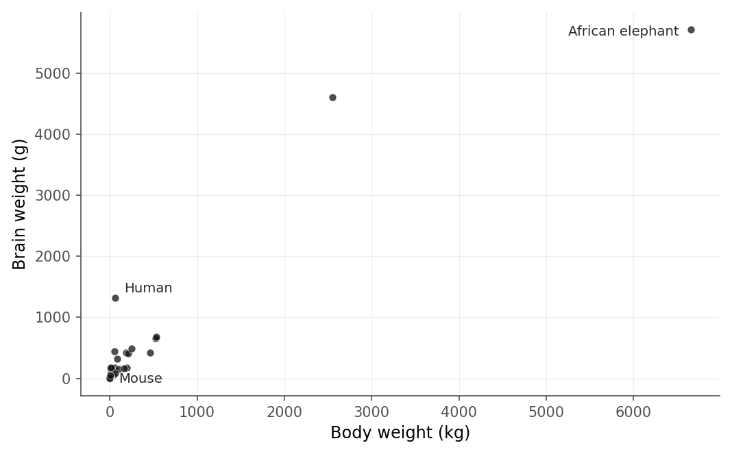
Figure 1:On the raw scale the mammal data are hopeless: most species pile up near zero while a few giants stretch the axes, and the vertical scatter grows with body size. No straight line summarizes this well.
Nothing is wrong with the data. What is wrong is the scale. Take the logarithm of both axes and the same 62 points snap into a clean, straight, evenly scattered band, shown in Figure 2. The relationship was always simple; it was simple in percentage terms, not in raw grams and kilograms, and the log scale is where percentages live. This is the central move of the chapter. When the diagnostics of Chapter 9 fire, you rarely need to abandon regression. More often you need to fit it to a transformed version of the problem, or weight the observations, or replace the loss function, so that the model’s assumptions become true.
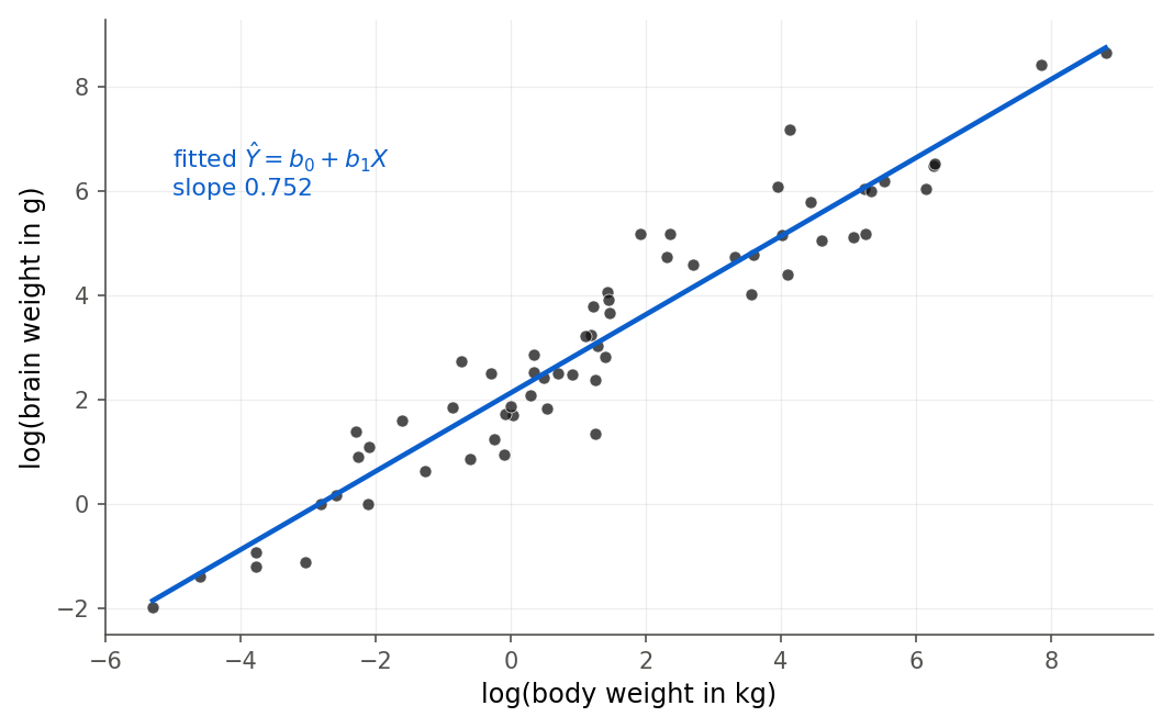
Figure 2:The same data on the log-log scale: a straight line, even scatter, and one clear slope near 0.75. Taking logs of both variables turned a hopeless plot into a textbook regression.
Chapter 9 taught you to detect trouble: curved residual plots, funnel shapes, heavy tails, one island or one country bending the whole fit. This chapter is the toolbox of fixes. You will read log coefficients as percentages, pick a transformation with the Box-Cox likelihood, weight observations that carry unequal noise, and resist a stubborn outlier with robust regression. At the end you will meet a dataset that no transformation can save, and learn to recognize when the honest fix is a different model entirely.
10.1 A menu of remedies
Before any single technique, it helps to see the whole menu and the logic that picks among its items. Chapter 9 ended by naming problems, from curved residual plots and funnel-shaped scatter to the high-leverage cases of 9.3 Influence: which points actually change the fit. Each named problem has a matching family of fixes.
If the residual plot curves, the mean function is wrong: a straight line is being asked to trace a bend. The fix is to bend the model back straight, either by transforming the predictor (leaving the error alone) or by transforming the response . If the residual plot fans out, the variance is not constant: the model assumes one but the data carry more noise in some places than others. The fix is either a variance-stabilizing transformation of or weighted least squares, which tells the fit to trust the low-noise points more. If the residuals have heavy tails or a lone outlier, one or two points are dominating the squared-error loss. The fix is a loss that grows more slowly than the square, which is robust regression. And if the response is a count, a proportion, or a strictly positive amount with structural skew, the normal-errors model may be the wrong frame altogether, and the fix is a different model, which is where Chapters 13 and 14 go.
The whole logic fits on one page. Figure 3 lays it out as a decision chart: start at the residual plot, read the pattern, and follow the arrow to the fix. Keep it beside you for the rest of the chapter, which walks the four columns from left to right.
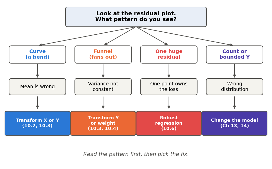
Figure 3:The remedy map for the whole chapter: the shape in the residual plot points to the fix. Read the pattern first, then pick the tool, and follow the section numbers to the details.
Transformations of the predictor and the response do different jobs, and it is worth keeping them apart. Transforming changes the shape of the mean curve without touching the errors, so it is the tool for a curved relationship whose scatter is already even. Transforming changes both the shape and the spread at once, so it is the tool when a curve and a funnel appear together, exactly as in the mammal data. A rough guide, drawn in Figure 4, is the “ladder of powers”: if a plot bends one way, step down the ladder from toward , , ; if it bends the other way, step up toward . The Box-Cox method in 10.3 Box-Cox: letting the data choose the power turns this guessing into an estimate.
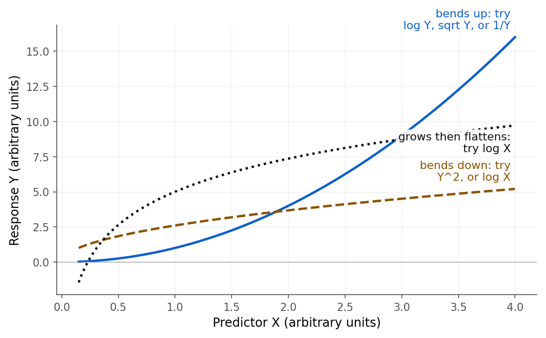
Figure 4:The ladder of powers as a decision aid: the direction a curve bends points to the transformation that straightens it. Bends upward call for pulling the response down the ladder; bends that flatten call for compressing the predictor.
The rest of the chapter takes these remedies one at a time. Throughout, keep the Chapter 2 model in view: with errors that should average to zero, share one variance , and be uncorrelated. Every remedy here is an effort to make one of those three conditions true after a diagnostic showed it was false.
10.2 The log transformation and reading its coefficients
The log transformation earns its own section because it is the most common remedy and the one most often misread. We can now fit the mammal line; the harder question is what its slope of 0.75 actually means, because a coefficient on a logged variable is not a change in grams per kilogram. It is a percentage.
Intuition
Logarithms turn multiplication into addition, so they turn “grows by a percentage” into “grows by a constant.” A quantity that doubles every time some driver doubles looks curved on ordinary axes and straight on log axes. Brain weight relates to body weight that way: across species, a body ten times heavier tends to carry a brain a fixed multiple larger, not a fixed number of grams larger. That is why the raw plot curved and the log-log plot is straight. The price of the straight line is that the slope now speaks in percents, and you have to translate.
Formula
Two log models cover almost every case. The log-log model logs both sides,
and the log-linear model logs only the response,
Here is the natural logarithm (base ) throughout this book. The slope means something different in each model, and each meaning carries a name (Definition 10.1, Definition 10.2).
In words: on the log-log scale the slope answers “if rises 1%, about how many percent does rise,” and on the log-linear scale it answers “if rises by one of its own units, about how many percent does rise.” Both readings have an exact form and an approximate form, and the next derivation produces both.
Derivation (exact and approximate percent readings)
Proof. Undo the log on the response. The log-log model says for the mean, so exponentiating,
In words: the mean of is a constant times a power of . Now multiply by a factor (for a 1% increase, ; for a doubling, ). The new mean divided by the old is
So multiplying by multiplies by , exactly. The exact percent change in for a 1% rise in is . For the approximate reading, use when is small; with , , giving a percent change of about percent. That is the elasticity headline: on the log-log scale, is roughly the percent change in per percent change in .
Proof (log-linear semi-elasticity). In the log-linear model the mean satisfies , so . Raise by one unit:
So each one-unit step in multiplies by , exactly, giving an exact percent change of . Since for small , the approximate percent change is percent per unit.
The gap between exact and approximate widens as the coefficient grows, drawn in Figure 5. For a coefficient near the two agree to a rounding error, which is why the “percent per unit” shortcut is safe for small effects and misleading for large ones. This same machinery returns twice later: as the odds ratio in logistic regression (13.3 Reading coefficients as odds ratios) and as the percent growth per month in the logged airline series (15.5 Forecasting honestly: test on the future).
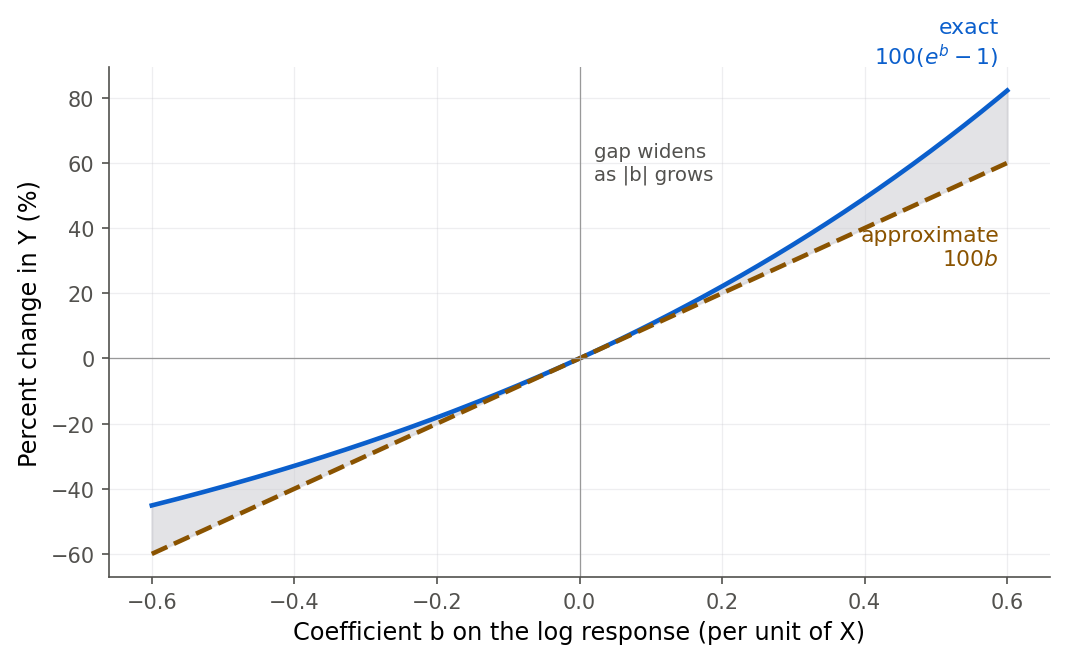
Figure 5:The exact percent reading and the linear approximation agree near zero and drift apart in the tails. Below about 0.1 in magnitude the shortcut is fine; past that, use the exact factor.
R
The mammal fit is a log-log model, so its slope is an elasticity.
mammals <- read.csv("data/mammals.csv")
dim(mammals)
head(mammals, 3)
[1] 62 3
species body brain
1 Arctic fox 3.385 44.5
2 Owl monkey 0.480 15.5
3 Mountain beaver 1.350 8.1The fastest way to feel why an elasticity is a percentage is to set one yourself and read the translation as it changes.
Set the intercept and the elasticity for the 62 mammals on the log-log scale, and watch the exact and approximate percent readings of Theorem 10.3 update with every step.
What to notice. The exact reading and the shortcut never part company by more than a tenth of a point anywhere on the slider, which is exactly what the derivation promises for a small coefficient. Try this. Push down from 1 until SSE stops falling, land near 0.75, and read off the percent that 10.2 The log transformation and reading its coefficients asks you to report.
10.3 Box-Cox: letting the data choose the power
Guessing a transformation from the ladder of powers works, but it feels arbitrary, and
two analysts can disagree. Box and Cox proposed a principled fix: put the candidate powers
into one family indexed by a number , then let maximum likelihood pick the
that makes the normal model fit best. We can now motivate the method with a
dataset that curves and fans at once: the classic cars data, where a car’s stopping
distance is measured against its speed.
Intuition
The powers , , , and are all special cases of raising to a power. If you write the transformation as one smooth function of a power parameter , then choosing a transformation becomes choosing a number, and choosing a number is something likelihood does well. Box-Cox writes down the likelihood of the data as a function of , with the regression coefficients and error variance profiled out, and reports the that maximizes it, plus a confidence interval so you know how sharply the data pin it down.
Formula
is the power parameter to be estimated; is essentially no transformation, is the square root, is the log, is the reciprocal.
The “-1” and division by make the family continuous at , where it becomes , so the ladder has no gap.
In words: one dial slides smoothly through all the rungs of the ladder of powers, and the log sits exactly at the notch.
Derivation (Box-Cox as a profile likelihood)
Proof. Assume that for the correct power the transformed response follows the normal linear model,
where is the -th row of the design matrix from 7.1 The model and least squares in matrix form. In words: once is raised to the right power, the result obeys the ordinary normal regression model. The parameters are , , and . The subtle point is that the likelihood must be written for the original data , not for the transformed , because we are comparing different values of and each puts on a different scale. Changing variables from to brings in the Jacobian, the derivative factor that any change of variables introduces, here . The log-likelihood of the observed is therefore
In words: this is the usual normal log-likelihood for the transformed response, plus one extra term that corrects for stretching the scale (the sum of the log-Jacobians). Now profile out and : for any fixed , the values that maximize are exactly the least-squares fit of on , giving residual sum of squares and (the same argument as the normal maximum-likelihood estimate of the variance in Chapter 2). Substituting these back and dropping constants leaves the profile log-likelihood, a function of alone:
In words: for each , fit the transformed response by ordinary least squares, read off its residual sum of squares, penalize by the Jacobian term, and the best is the one that maximizes the result. The maximizer is the Box-Cox estimate. A % confidence interval is the set of with , the usual likelihood-ratio interval.
R
R’s MASS::boxcox computes over a grid and draws it. The plot in
Figure 8 is the profile log-likelihood for the cars model, with its peak
and 95% interval marked.
cars <- read.csv("data/cars.csv")
fit_lin <- lm(dist ~ speed, data = cars)
coef(fit_lin)
(Intercept) speed
-17.579095 3.932409The straight-line fit is not obviously wrong, but its residuals fan out as the fitted distance grows, the funnel shown in Figure 7. That widening scatter is the signal that the response needs a transformation, and Box-Cox will say which one.
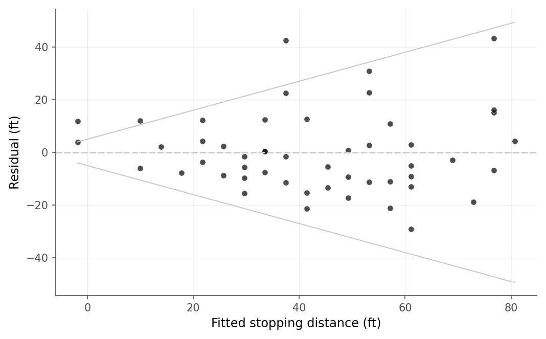
Figure 7:The residuals from the raw linear fit of stopping distance on speed fan out as the fit grows: small scatter for slow cars, large scatter for fast ones. This funnel is the nonconstant-variance warning that motivates transforming the response.
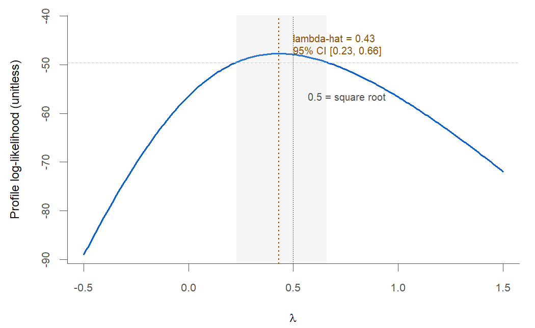
Figure 8:The Box-Cox profile for the cars data peaks at lambda about 0.43, and the 95 percent interval runs from 0.23 to 0.66. Because 0.5 sits comfortably inside, the square-root transformation is a clean, interpretable choice.
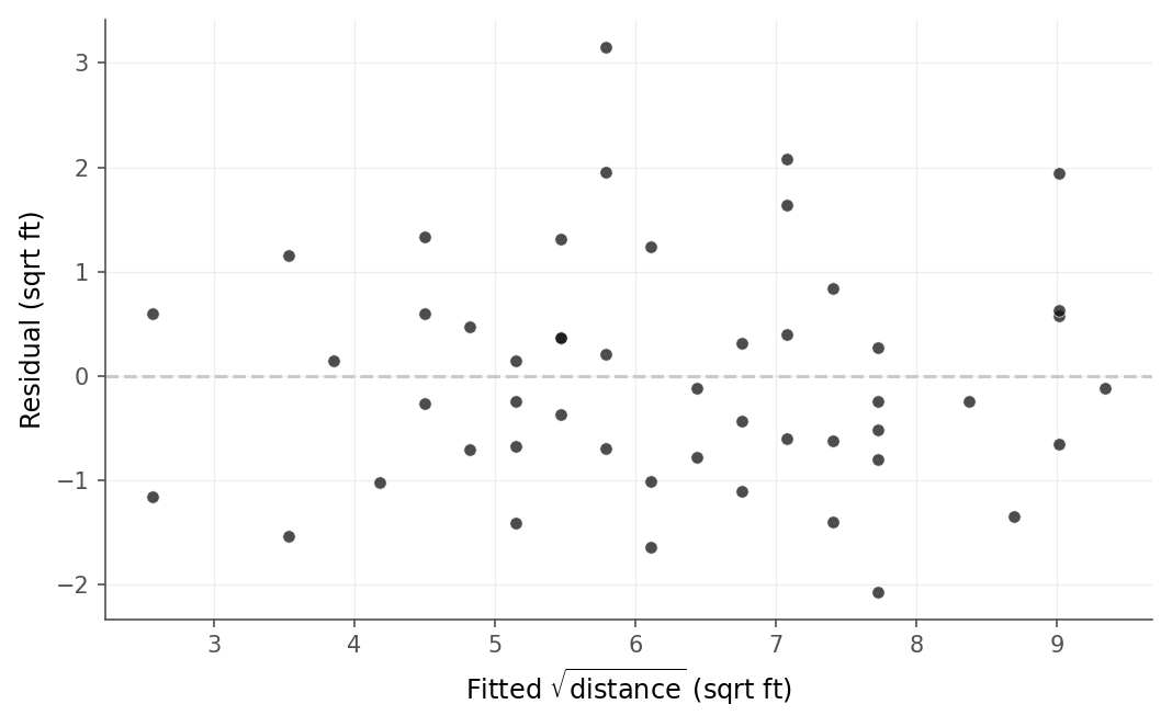
Figure 9:After the square-root transform the residual funnel from the raw fit is gone: the scatter is now an even band around zero. The transformation stabilized the variance and straightened the mean at once.
The profile likelihood is easier to trust once you have watched it fight the residual plot for a while, so take the dial yourself.
Move through the Box-Cox family and the 50 cars are refitted from scratch, so the residual funnel of Figure 7 reshapes live while , , and track it.
What to notice. The profile log-likelihood and the shape of the residual plot agree: climbs from -135.63 at to its peak -126.73 at exactly as the funnel flattens, and alone would have told you nothing, since it falls all the way to 9.56 at the log. Try this. Find the peak by hand, then keep going down past and watch a new low outlier open up, the picture of over-transforming that 10.3 Box-Cox: letting the data choose the power warns about.
10.4 Weighted least squares
Transformations attack a curved mean or a variance that grows with the mean. Sometimes, though, the variance is unequal for a reason that has nothing to do with the mean: some observations are simply measured more precisely than others. Averaging ten readings gives a more reliable point than a single reading; a well-calibrated instrument beats a rough one. When you know the relative precision of each point, you should not throw that knowledge away by treating every point equally. Weighted least squares is how you use it.
Intuition
Ordinary least squares gives every observation the same vote. If one point carries ten times the variance of another, that is like letting a noisy witness testify as loudly as a careful one. Weighted least squares turns down the volume on the noisy points and turns it up on the precise ones, in exact inverse proportion to their variances. Figure 11 shows the idea: low-noise points are drawn large because they count more.
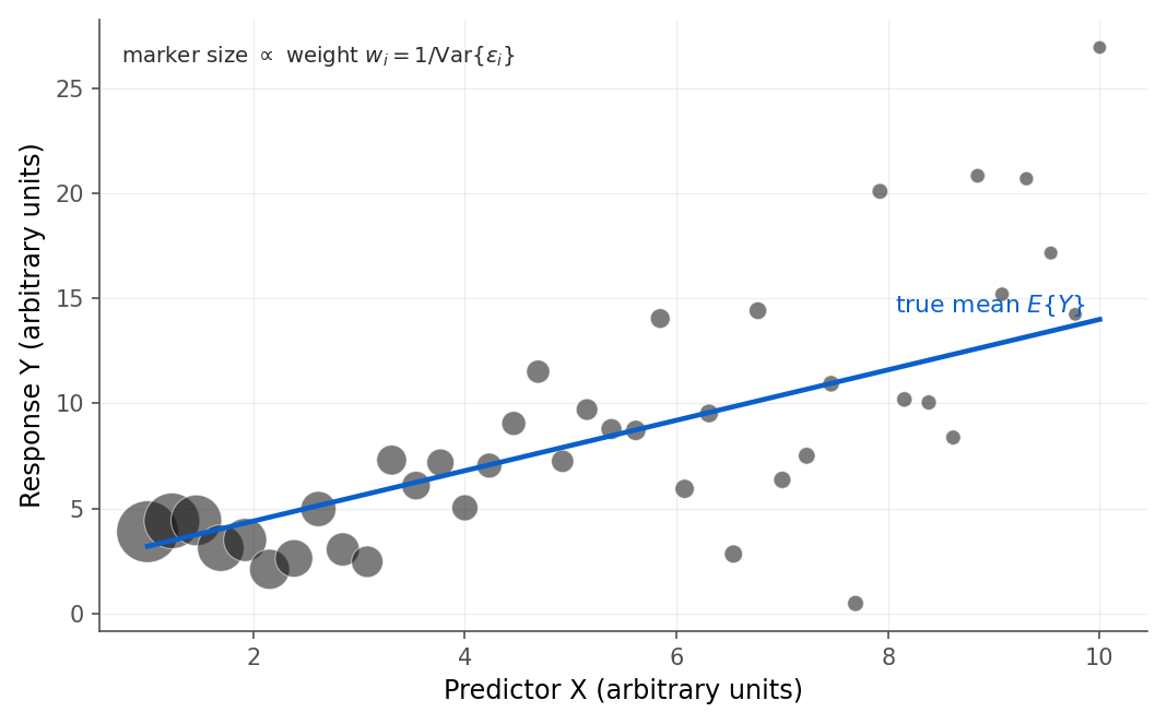
Figure 11:Weighted least squares gives each point influence in inverse proportion to its variance. The precise, low-noise points (drawn large) pull harder on the line than the noisy ones (drawn small).
Formula
Keep the linear model but let the error variances differ:
Here is known up to the common constant .
In words: penalize each squared residual by its weight, so precise points contribute more to the total the fit is trying to shrink.
Derivation (WLS from Gauss-Markov)
Proof. The trick is to transform the unequal-variance model into an equal-variance one and then quote the Gauss-Markov result we already proved. Multiply the -th observation through by . Collecting these into matrices with , define
The transformed model is , and its errors are now homoscedastic:
The starred model satisfies every ordinary least squares assumption, so by the matrix Gauss-Markov theorem (7.6 The Gauss-Markov theorem) the best linear unbiased estimator is ordinary least squares on the starred data:
This is the WLS estimator, and because it is OLS on a model that truly has constant variance, it inherits every good property: it is unbiased and it is BLUE, with . Plain OLS on the original data is still unbiased here, but it is no longer best: it wastes the precision information in the weights.
The derivation also tells you how to compute WLS with nothing but an OLS routine: form and and regress. We use that as a check below.
R
The strongx data are a physics experiment: at ten beam energies, a scattering
cross-section was measured, and each measurement comes with its own known standard
deviation sd. Known standard deviations are the textbook case for WLS, with weights
.
strongx <- read.csv("data/strongx.csv")
strongx[, c("energy", "crossx", "sd")]
energy crossx sd
1 0.345 367 17
2 0.287 311 9
3 0.251 295 9
4 0.225 268 7
5 0.207 253 7
6 0.186 239 6
7 0.161 220 6
8 0.132 213 6
9 0.084 193 5
10 0.060 192 5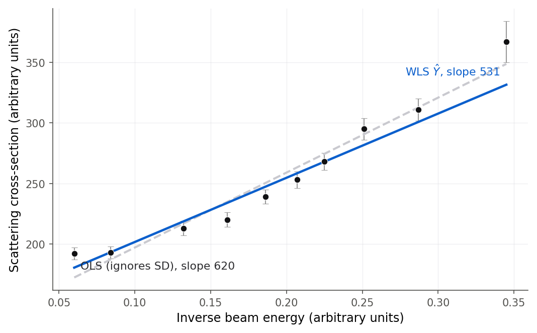
Figure 12:The strongx measurements with their known error bars, fit two ways. WLS (solid) leans toward the precise, small-error-bar points, while OLS (dashed) treats every point equally and is pulled by the noisier ones.
When the variances are not known, you estimate the weights, usually by modeling how the spread grows (for example, regressing the absolute residuals on a predictor and using the fitted values to build weights). That two-step method, iterated, is common and effective, and it recycles the variance-modeling instinct that Chapter 14 reuses to handle overdispersion in count models. The strongx case is cleaner because physics handed us the variances directly.
Weights are easiest to believe when you can turn them up gradually and watch the line answer, so slide between ordinary and weighted least squares yourself.
The slider sets how hard the known precisions push, from where every strongx measurement votes equally to where the weight is the textbook .
What to notice. At the weighted line sits exactly on the ordinary one, which is the derivation’s statement that equal weights give back plain least squares. Try this. Raise to 1 and watch the slope fall from 619.7 to 530.8 while drops from 10.08 to 8.08: the numbers of Example 10.3, arriving as a rotation you can see. Keep going to and ask yourself whether you would still trust a fit resting on so few points (10.4 Weighted least squares).
10.5 When a transformation is not enough: the Galapagos counts
Every remedy so far assumed the underlying model was sound and only its scale or its weighting was off. Sometimes that assumption is wrong, and a transformation only hides the problem. The Galapagos species data from Chapter 9 are a case in point, and following them here shows you how to tell a fixable scale problem from a model that needs replacing.
Recall the setup from 9.3 Influence: which points actually change the fit: for 30 Galapagos islands, the number of plant species is regressed on geographic predictors (area, elevation, and distances), and one island, Isabela, has an enormous leverage value because it dwarfs the others in area. The raw fit has a residual funnel, because islands with more species also scatter more widely, the signature of count data. A natural remedy is a variance-stabilizing transformation. For counts, the square root is the classic choice, since a Poisson count with mean has variance , and has roughly constant variance.
gala <- read.csv("data/gala.csv")
fit_g_lin  <- lm(Species ~ Area + Elevation + Nearest + Scruz + Adjacent,
                 data = gala)
fit_g_sqrt <- lm(sqrt(Species) ~ Area + Elevation + Nearest + Scruz + Adjacent,
                 data = gala)
round(c(R2_linear = summary(fit_g_lin)$r.squared,
        R2_sqrt   = summary(fit_g_sqrt)$r.squared), 4)
R2_linear R2_sqrt
0.7658 0.7827The square root helps a little, and Figure 14 shows the funnel easing. But look closer and the cracks show. Isabela still has a leverage value of 0.97 on the transformed fit, essentially unchanged, because transforming does nothing about an that is far from the others.
h <- hatvalues(fit_g_sqrt)
names(h) <- gala$island
round(sort(h, decreasing = TRUE)[1:3], 3)
Isabela Fernandina Darwin
0.969 0.950 0.466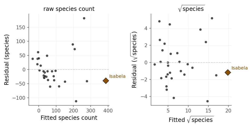
Figure 14:Transforming the response eases the funnel (right panel versus left) but leaves Isabela’s influence intact, because a square root of the response cannot fix a predictor value that is extreme. The transformation treated a symptom, not the cause.
Figure 15 shows why the gap opens, using the squaring curve that undoes a square-root fit. Take two predictions equal distances above and below the average. Squaring bends the curve upward, so the high one climbs more than the low one drops. Their average (on the straight chord) lands above the square of the average (on the curve), and that vertical gap is the bias. Any curved back-transform, including the log, does the same thing.
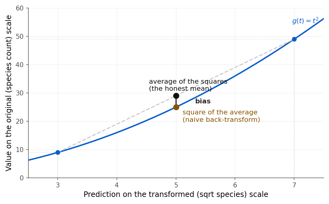
Figure 15:Because the back-transform curve bends upward, averaging along the chord lands above the curve. The square of the average (green) sits below the honest average of the squares (red), and that gap is the back-transformation bias.
Step back and count the warning signs. The response is a count. Several islands have very few species (six islands have fewer than ten). The variance grows with the mean by construction. Back-transformed predictions are biased, and a plain linear fit to the counts predicts a negative number of species for the smallest islands, which is impossible. Every one of these says the same thing: the normal, constant-variance linear model is the wrong frame, and no power of will make it right. The honest fix is not to transform the data until they fit the model, but to change the model to one built for counts. That model is Poisson regression, and 14.1 Why counts break the linear model returns to these exact islands and fits them properly, recalling both Isabela’s high-leverage status from Chapter 9 and this failed transformation. For now, the lesson is diagnostic: learn to tell a scale problem, which a transformation fixes, from a distributional problem, which it cannot.
10.6 A first look at robust regression
The last remedy addresses a different failure: not a curved mean or unequal variance, but a handful of points with outsized residuals that drag the fit toward themselves. Least squares is exquisitely sensitive to such points because it squares residuals, so a single large one can dominate the entire sum. Robust regression replaces the square with a loss that grows more gently, so no one point can take over.
Figure 16 shows the payoff on a simple cloud with one point knocked far off. The least-squares line tilts up to chase the stray point; the Huber line shrugs it off and stays with the crowd. That is the entire promise of robust regression in one picture, and the rest of the section explains how the capped loss delivers it.
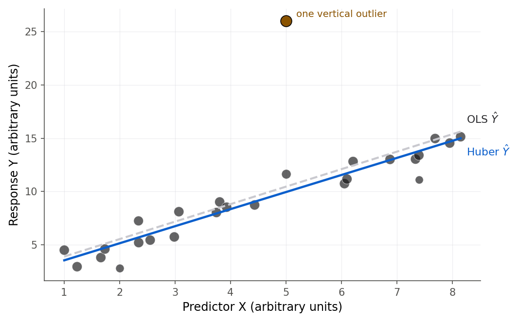
Figure 16:One vertical outlier, two fits. Ordinary least squares (dashed) is dragged toward the stray point, while the Huber fit (solid) keeps to the bulk of the data. The capped Huber loss limits how hard any single point can pull.
Intuition
Picture the sum of squared residuals as a tug of war in which each point pulls with a force proportional to its residual. A point twice as far off pulls four times as hard, because of the square. Huber’s idea is to cap that escalation: inside a normal range, keep the squared loss and its efficiency, but once a residual is large enough to look like an outlier, let its pull grow only linearly, not quadratically. Figure 17 draws the resulting weight each point receives.
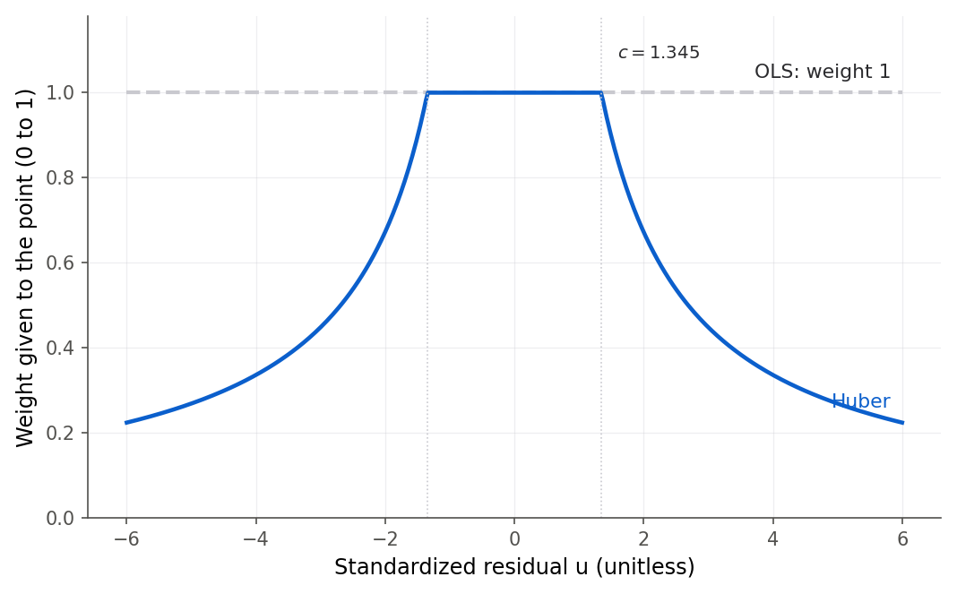
Figure 17:The Huber weight function keeps full weight 1 for residuals inside a central band and then tapers off like 1 over the residual size beyond it. OLS, by contrast, gives every point full weight no matter how extreme.
Formula
M-estimation, where the M signals a maximum-likelihood-style objective, replaces the least-squares objective with
where is the Huber loss.
is the residual standardized by a resistant scale estimate .
is a tuning constant; gives about 95% of the efficiency of OLS when the errors really are normal, while bounding the influence of outliers.
In words: penalize ordinary residuals by the familiar square, but penalize far-out residuals only linearly, so an outlier is expensive rather than catastrophic.
Derivation (IRLS and the honest limitation)
Proof. Differentiate the objective and set it to zero. With , the estimating equations are . Write with the weight
Then the estimating equations become , which are exactly the weighted least squares normal equations from 10.4 Weighted least squares with weights . The catch is that the weights depend on the residuals, which depend on the fit. So we iterate: start from the OLS fit, compute residuals and hence weights, solve the WLS problem, recompute residuals and weights, and repeat until the coefficients stop moving. This is iteratively reweighted least squares (IRLS). A residual inside the band () keeps weight 1; a wild residual gets weight , shrinking as it grows.
The derivation exposes the method’s honest boundary. The weight depends only on the residual, so Huber regression protects against outliers in the response direction, points with a large vertical miss. It does nothing about a point whose predictor values are extreme, a high-leverage point, unless that point also happens to have a large residual. A high-leverage point often pulls the line onto itself and so keeps a small residual, sailing through with full weight. Guarding against that needs a bounded-influence or MM-estimator, which we do not develop here. The savings data make the limitation concrete.
R
Fit the Chapter 8 savings model both ways, ordinary and Huber, on the 50 countries.
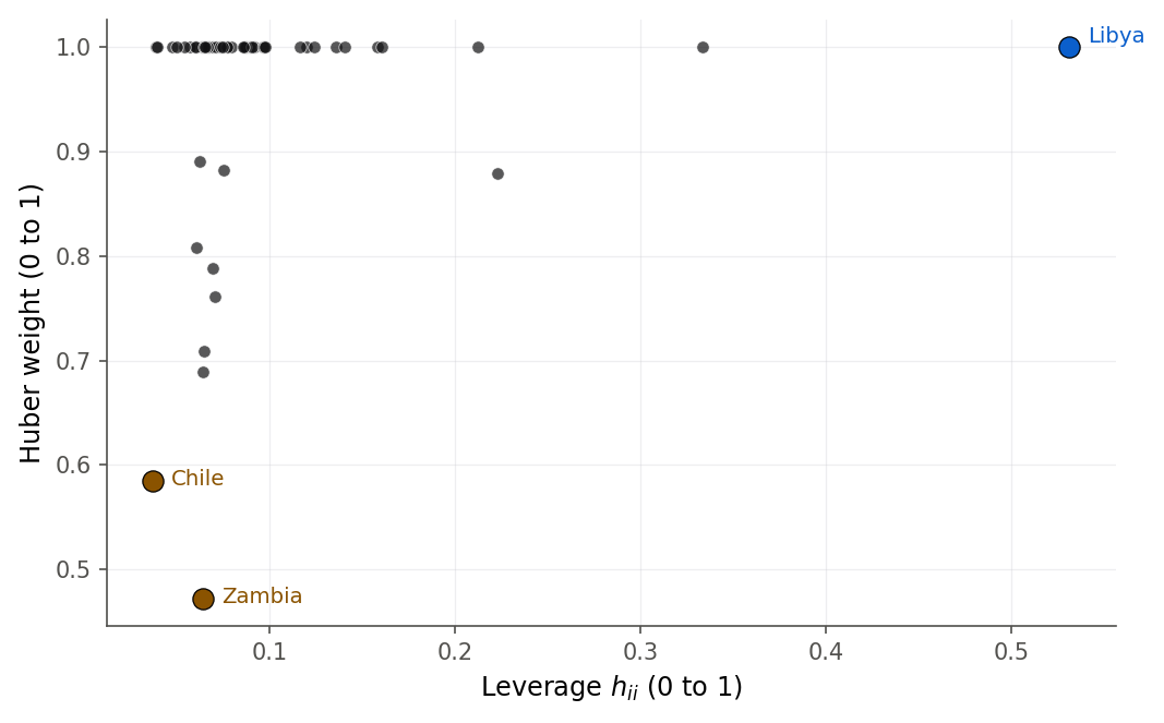
Figure 18:Huber weight against the leverage value for the savings countries. Huber downweights the large-residual points (Zambia, Chile) but leaves the highest-leverage point, Libya, at full weight, exactly the blind spot the derivation predicts.
10.7 Chapter summary
You can now respond to a failed diagnostic instead of just naming it. You read a menu of remedies and match each to the pattern that calls for it: transform the predictor for a curved mean with even scatter, transform the response for a curve and a funnel together, weight for known unequal precision, use a slower-growing loss for vertical outliers, and change the model when the response is a count or a proportion. You interpret log coefficients as percentages on both the exact and the approximate scale, choose a power with the Box-Cox profile likelihood and its confidence interval for , derive weighted least squares from the Gauss-Markov argument and compute it from known weights, and read Huber regression as iteratively reweighted least squares while stating its honest limitation. And you can recognize, as with the Galapagos counts, when no transformation will do and a different model is the right answer.
Key results at a glance
| Result | Statement or formula | Valid when |
|---|---|---|
| Log-log elasticity (Theorem 10.3) | multiplies by ; a 1% rise in gives in | log-log model, mean |
| Log-linear semi-elasticity (Theorem 10.4) | one unit of multiplies by ; exact percent | log-linear model, mean |
| Box-Cox family (Definition 10.5) | , at | positive response |
| Box-Cox profile log-likelihood (Theorem 10.6) | transformed obeys the normal linear model | |
| Weighted least squares (Definition 10.7, Theorem 10.8) | is BLUE, | , weights known |
| Huber loss (Definition 10.10) | quadratic for $ | u |
| Huber estimating equations (Theorem 10.11) | , $w(u) = \min(1, c/ | u |
Key terms. Remedial measure, log-log model, log-linear model, elasticity, semi-elasticity, Box-Cox family, profile likelihood, Jacobian term, weighted least squares, weight, whitening, back-transformation bias, robust regression, M-estimation, Huber loss, iteratively reweighted least squares.
You should now be able to
Choose a remedy (transform , transform , weight, or change the model) from the diagnostic pattern you see.
Interpret a log-transformed coefficient on both the exact and the approximate percent scale, and derive both readings.
Derive the Box-Cox profile log-likelihood, including the Jacobian term, and use it to pick a response transformation with a confidence interval for .
Derive weighted least squares from the Gauss-Markov argument and compute it from known weights.
Explain and demonstrate Huber robust regression, and state what it protects against and what it does not.
Decide when a transformation is a patch and a different model is the honest fix.
Where this fits. In the workflow spine of The modeling workflow, this chapter lives at the seam between CHECK and FIT. Chapter 9 (CHECK) told you an assumption was broken; the remedies here send you back to FIT with a better-specified model, a transformed scale, or a weighting scheme, after which you CHECK again and only then USE the result. That loop, diagnose then remedy then re-diagnose, is the working core of applied regression, and it rarely ends after one pass. The threads continue: the log-interpretation machinery of 10.2 The log transformation and reading its coefficients returns as odds ratios in 13.3 Reading coefficients as odds ratios and as monthly growth in 15.5 Forecasting honestly: test on the future, the variance-modeling instinct of 10.4 Weighted least squares returns as overdispersion in 14.6 One family: the generalized linear model, and the Galapagos islands that defeated every transformation here get their honest resolution in 14.1 Why counts break the linear model.
10.8 Frequently asked questions
Q1. Should I transform , transform , or both? Look at the residual plot. A curved mean with even scatter is a predictor problem: transform and leave the errors alone. A curve together with a funnel is a response problem: transform , which fixes both at once. When only the variance fans out but the mean is straight, prefer weighting or a variance-stabilizing transform of . The mammal data needed both variables logged because the relationship was multiplicative in both.
Q2. When is the “percent per unit” shortcut safe? When the coefficient is small in magnitude, roughly under 0.1. Then the exact factor and the approximation agree to a fraction of a percent (Figure 5). For a coefficient like 0.5 or larger, report the exact percent , since the shortcut can be off by several points.
Q3. Box-Cox gave . Why did we use instead? Because 0.5 is inside the 95% confidence interval , so the data do not distinguish it from the maximum, and the square root is far easier to interpret and to justify than a raw power of 0.43. Round to a nearby interpretable value whenever the interval allows it.
Q4. My response has zeros or negatives. Can I still use Box-Cox or a log? Not directly: both need . Common fixes are a small shift () or, better, a model built for the data type, since zeros in a count or a proportion usually signal that a generalized linear model (Chapters 13 and 14) is the right tool, not a shifted transform.
Q5. If OLS is unbiased even under unequal variances, why bother with WLS? OLS stays unbiased but stops being efficient: it no longer has the smallest variance, and its reported standard errors are wrong because they assume one common . WLS restores both the efficiency and the honest standard errors by using the known precision of each point, as the strongx intercept’s tighter standard error showed.
Q6. Does robust regression replace diagnostics? No. It guards against vertical outliers automatically, but it is blind to high-leverage points (the Libya lesson), and its standard errors are approximate. Use it as one tool alongside the Chapter 9 diagnostics, and always investigate why a point is unusual before deciding to downweight it. A downweighted point is sometimes the most interesting observation in the data.
Q7. How do I get a prediction on the original scale from a transformed model? Undo the transform, but know that naively back-transforming the fitted value is biased, as squaring Isabela’s prediction overshot by 46 species. The mean of a nonlinear function is not that function of the mean. For the log model there is a standard smearing correction; for careful prediction intervals, transform the interval endpoints rather than the point estimate.
10.9 Practice problems
(A) For each diagnostic pattern, name the remedy this chapter recommends: (i) a curved residual plot with even scatter; (ii) a curve and a funnel together; (iii) a single point with a huge residual; (iv) a count response with many small values.
(A) Explain the difference between transforming a predictor and transforming the response in terms of what each does to the mean function and to the error variance.
(A) A log-log model has slope . State in words what a 1% increase in does to , and whether grows more or less than proportionally.
(A) Distinguish an elasticity from a semi-elasticity, and say which log model produces each.
(A) In the Box-Cox family, what transformation does each of correspond to? Why is the family written with the “-1” and the division by ?
(A) Explain in one or two sentences why the Box-Cox profile log-likelihood includes the Jacobian term , and what goes wrong without it.
(A) State the weighted least squares criterion in words, and explain why a point with small variance should get a large weight.
(A) Why does ordinary least squares remain unbiased under unequal error variances but stop being the best linear unbiased estimator?
(A) Describe the difference between a vertical outlier and a high-leverage point, and say which one Huber regression protects against.
(A) Give two features of a response variable that should push you toward a different model rather than a transformation, and name the chapter that supplies that model.
(B) Starting from the log-log mean relation , derive that multiplying by multiplies by exactly (Theorem 10.3), and derive the approximate “ percent per percent” reading.
(B) For the log-linear model, derive the exact factor per unit of and its approximation , and find the coefficient value at which the approximation understates the true percent change by exactly one percentage point.
(B) Derive the Box-Cox profile log-likelihood (Theorem 10.6) from the full log-likelihood, showing how and are profiled out and where the Jacobian term comes from.
(B) Show that the Box-Cox family is continuous at , that is, .
(B) Derive the weighted least squares estimator (Theorem 10.8) by transforming the model with and applying the Gauss-Markov theorem. State the variance of .
(B) Show that WLS minimizes by differentiating and obtaining the weighted normal equations .
(B) For simple linear regression through weighted least squares, derive the closed form , where and are the weighted means. Define the weighted means.
(B) Starting from the Huber loss (Definition 10.10), compute and show that the estimating equations can be written as weighted normal equations with weight (Theorem 10.11).
(B) Explain, using the weight , why a high-leverage point with a small residual is not downweighted by Huber regression. Contrast with a low-leverage point that has a large residual.
(B) Suppose row of a dataset is the average of independent readings each of variance . Show that the correct WLS weight is , and identify the common constant in the model .
(C) Fit the mammal log-log model in R or Python, report , , and , and translate the slope into the exact percent change in brain weight for a 25% increase in body weight.
(C) Using
cars.csv, reproduce the Box-Cox estimate and its 95% interval, then fit bothdist ~ speedandsqrt(dist) ~ speedand compare their residual-versus-fitted plots. Which model better satisfies constant variance?(C) Using
strongx.csv, fit OLS and WLS with weights , report both slopes and both intercept standard errors, and confirm the WLS coefficients by regressing the -scaled variables with no intercept.(C) On
strongx.csv, add a quadratic term (crossx ~ energy + I(energy^2)) to the WLS fit and compare it to the linear WLS fit. Does the curvature term improve the fit, and what does that say about the linear model?(C) Using
gala.csv, fitSpeciesandsqrt(Species)on the five geographic predictors, compare and the residual plots, and report Isabela’s leverage value in both fits. Explain why the transformation does not reduce Isabela’s leverage value.(C) Predict the species count for Fernandina from the square-root gala model, back-transform by squaring, and compare to its actual count. Comment on the direction of the back-transformation bias.
(C) Using
savings.csv, fit OLS and Huber regression ofsron the four predictors, list the four countries with the smallest Huber weights, and cross-tabulate each against its leverage value. Identify a high-leverage country that Huber does not downweight.(C) Simulate heteroscedastic data (seed 4210): 40 points with proportional to , fit OLS and WLS with weights , and compare the two slope estimates and their standard errors across 500 replications. Which is more precise, and does either show bias?
10.10 Exam practice
These five questions are written in the style of the course exams: each asks you to
explain, evaluate, or interpret in full sentences, not just to produce a number. Where a
question shows software output, the numbers were produced on the course machine (R 4.6.0)
reading the same CSV files from data/ you used all term; Python with statsmodels gives
the same values. Read the output, then answer in complete sentences with units. Try each
question before opening its model answer.
EP 10.1 (evaluate a claim). A classmate fits a log-linear model of Galapagos plant species on island elevation and reads the slope as a percent effect.
gala <- read.csv("data/gala.csv")
fit <- lm(log(Species) ~ Elevation, data = gala)
round(coef(fit), 6)
(Intercept) Elevation
2.591399 0.002490The classmate writes: “The coefficient 0.00249 means about more species per meter of elevation, so an island 100 meters higher has about more species.” Explain what the coefficient means on the percent scale, then evaluate both readings: the per-meter one and the 100-meter one. Which is sound, which is not, and what is the correct figure for a 100-meter difference?
Model answer
In this log-linear model the slope is a semi-elasticity: the approximate percent change in species per one-unit (one-meter) change in elevation. The exact factor for one meter is , an exact percent change of , and the approximation agrees to three decimals. So the per-meter reading is sound, because the coefficient is tiny and the exact and approximate readings coincide.
The 100-meter claim is where the classmate slips. A 100-meter rise is not a small change, and you cannot get its effect by multiplying the per-meter percent by 100, because percent changes compound rather than add. The correct exact figure raises by 100 units, which multiplies species by , an increase of , not . The classmate’s is the linear approximation , which understates the true effect by about 3.4 percentage points. The gap is exactly the exact-versus-approximate spread of Figure 5: harmless for a one-meter step, real once the change is large enough that the exponent is no longer near zero.
A weak answer stops at “about per meter” and repeats it as over 100 meters, missing that a large change needs the exact factor and that percent effects compound.
EP 10.2 (interpret output in context). Box-Cox run on the raw mammal regression of brain weight on body weight returns the output below.
mammals <- read.csv("data/mammals.csv")
library(MASS)
bc <- boxcox(lm(brain ~ body, data = mammals),
             lambda = seq(-0.5, 0.5, by = 0.01), plotit = FALSE)
lambda_hat <- bc$x[which.max(bc$y)]
ci <- range(bc$x[bc$y > max(bc$y) - 0.5 * qchisq(0.95, 1)])
round(c(lambda_hat = lambda_hat, ci_low = ci[1], ci_high = ci[2]), 3)
lambda_hat ci_low ci_high
0.07 -0.03 0.18Interpret and its interval in context. Which transformation of the response does the output recommend, and why? The chapter’s opening logged both brain and body weight; does this Box-Cox result, which transforms only the response, justify that whole log-log move? Explain what Box-Cox does and does not tell you here.
Model answer
The estimate is with a 95% confidence interval . Because that interval contains 0, the log transformation () is fully supported by the data, and the log is far easier to read and to justify than a raw power near 0.07. So the output recommends modeling : report the log.
The important qualification is that Box-Cox chooses only the response transformation. It searches over powers of to make the errors of a fixed linear model in look normal and constant-variance; it says nothing about the predictor. Body weight is itself extremely right-skewed, running from a few grams to several tons, so even after logging brain weight a plot of against raw body weight still curves and lets a handful of giants stretch the horizontal axis and carry extreme leverage values. Logging body weight as well is what straightens the mean and evens out those leverage values, which is why the chapter fit the log-log model.
So this result justifies logging and is consistent with the log-log fit, but the decision to log is a separate one, driven by the predictor’s skew and the shape of the scatter, not by this profile likelihood. A weak answer reads “ near 0, so use the log” and stops, treating Box-Cox as if it had endorsed logging both variables, when it can only speak to the response.
EP 10.3 (what would change if). A student fits weighted least squares to the strongx
physics data with weights , then multiplies every weight by 10 and
refits, expecting the line to “trust the precise points ten times more” and shift.
strongx <- read.csv("data/strongx.csv")
w <- 1 / strongx$sd^2
fit1 <- lm(crossx ~ energy, data = strongx, weights = w)
fit2 <- lm(crossx ~ energy, data = strongx, weights = 10 * w)
rbind(w = coef(fit1), tenw = coef(fit2))
c(se_energy_w = summary(fit1)$coef["energy", "Std. Error"],
  se_energy_10w = summary(fit2)$coef["energy", "Std. Error"])
(Intercept) energy
w 148.4732 530.8354
tenw 148.4732 530.8354
se_energy_w se_energy_10w
47.55 47.55The slope, the intercept, and the slope’s standard error are identical to the last digit shown. Explain why multiplying every weight by the same constant changes nothing you would report, referring to the WLS model . What single quantity does change, and why is it not a result?
Model answer
In weighted least squares only the relative weights matter. The model states , so each is known only up to the common unknown constant . Multiplying every weight by 10 is the same as dividing by 10: it describes the identical set of relative precisions, so it is the same model. In the estimator , replacing by puts a factor of 10 in both the inverse and the right-hand side, and the two cancel exactly, so is unchanged.
The standard error is unchanged for the same reason. From , scaling by 10 scales by , while the estimated scales by 10; the two factors cancel and the reported standard error, statistic, and interval all stay put.
The one quantity that moves is the residual standard error, the estimate of itself, which changes by a factor of . That is not a result you report, because in this model is defined only relative to the arbitrary scale of the weights; it is a nuisance parameter, not a scientific quantity. Everything a reader cares about, the coefficients and their uncertainty, is invariant. A weak answer says “the coefficients do not change” without explaining that weights enter only as relative precisions ( is identified only up to scale), or wrongly expects the standard errors to shift.
EP 10.4 (interpret output in context). The output below shows the fitted values from the plain linear regression of Galapagos plant species on the five geographic predictors, for the five islands with the smallest fitted values.
gala <- read.csv("data/gala.csv")
fit_lin <- lm(Species ~ Area + Elevation + Nearest + Scruz + Adjacent, data = gala)
pred <- predict(fit_lin)
head(data.frame(island = gala$island, actual = gala$Species,
                fitted = round(pred, 1))[order(pred), ], 5)
island actual fitted
Coamano 2 -36.4
Darwin 10 -9.0
Bartolome 31 -7.3
Gardner1 58 -4.0
Genovesa 40 -0.5Interpret this output in the context of choosing a remedy. What is impossible about these predictions, why does it happen, and what does it tell you about whether any transformation of the response could rescue the linear normal model? Name the honest fix and the chapter that supplies it.
Model answer
Five islands are given negative fitted species counts, from Coamano at -36.4 down to Genovesa at -0.5. That is impossible: a species count cannot be less than zero. Notice that several of these islands actually hold dozens of species (Gardner1 has 58, Genovesa 40), so the model is not just rounding small numbers below zero; its straight-line mean function genuinely extends past zero for islands whose predictor combination sits at the low end, because the normal linear model puts no floor under its mean.
This is not a scale problem, and no transformation of repairs it. A variance-stabilizing transform such as the square root or the log can flatten the residual funnel, but the deeper trouble is distributional: the response is a bounded count whose variance is tied to its mean by the Poisson distribution, and no power of turns a normal, unbounded, constant-variance model into one that respects the zero floor and the mean-variance link. When a linear fit predicts impossible values, that is the signal to change the model, not the scale.
The honest fix is Poisson regression, which models the log of the mean count and therefore can never predict a negative count; it is developed in 14.1 Why counts break the linear model, which returns to these exact islands. A weak answer notices the negative numbers but proposes patching them, “take a square root” or “truncate at zero,” missing that the failure is distributional rather than a matter of scale.
EP 10.5 (evaluate a claim). An analyst refits the savings model with Huber robust regression and tells a colleague: “The robust regression fit automatically downweights every unusual country, so I no longer need the Chapter 9 diagnostics.” The output lists the four highest-leverage countries with their Huber weights; for contrast, Zambia has a leverage value of 0.064 and Huber weight 0.472.
savings <- read.csv("data/savings.csv")
fit_ols <- lm(sr ~ pop15 + pop75 + dpi + ddpi, data = savings)
fit_hub <- MASS::rlm(sr ~ pop15 + pop75 + dpi + ddpi, data = savings)
h <- hatvalues(fit_ols); wt <- fit_hub$w
data.frame(country = savings$country, leverage_value = round(h, 3),
           huber_weight = round(wt, 3))[order(-h)[1:4], ]
country leverage_value huber_weight
Libya 0.531 1.000
United States 0.334 1.000
Japan 0.223 0.879
Ireland 0.212 1.000Evaluate the analyst’s claim using these numbers. Which country is the clearest counterexample, what general limitation of Huber regression does it expose, and what should the analyst still do?
Model answer
The claim is false. Huber weights depend only on the size of a point’s residual, through , and not at all on its leverage value. The three highest-leverage countries, Libya (0.531), the United States (0.334), and Ireland (0.212), all keep full weight 1.000, and even Japan, next in line, is barely touched at 0.879. Huber leaves the high-leverage points essentially alone, because a high-leverage point tends to pull the fitted line onto itself and so carries a small residual that the weight function never flags.
Libya is the clearest counterexample: it has the highest leverage value in the data yet weight 1.00, the very influential case that distorted the fit in 9.3 Influence: which points actually change the fit. Meanwhile Zambia, a low-leverage country (0.064) with a large vertical residual, is downweighted hard to 0.472, which is exactly what Huber is built to do. So Huber guards against vertical outliers but is blind to high-leverage points, and it cannot stand in for the leverage values and Cook’s distances of Chapter 9.
The analyst should still compute the Chapter 9 leverage values and Cook’s distances, look at why Libya is extreme before trusting any fit, and, if high-leverage influence is a real concern, reach for a bounded-influence or MM-estimator rather than plain Huber. A weak answer agrees that “robust regression handles the outliers” or simply restates that Huber is resistant, without noticing that the highest-leverage countries keep weight 1 and that a residual-based weight cannot see leverage values at all.
Chapter game
Resumen del capítulo (en español)
Cuando los diagnósticos del Capítulo 9 fallan, rara vez hay que abandonar la regresión: casi siempre basta con corregir la escala, ponderar las observaciones o cambiar la función de pérdida para que los supuestos del modelo se cumplan. Este capítulo reúne esas medidas correctivas.
La transformación logarítmica (log transformation) es la más común. En el modelo log-log, la pendiente es una elasticidad (elasticity): multiplicar por un factor multiplica por , de forma exacta, y una subida del 1% en eleva en aproximadamente por ciento. Para los mamíferos, la elasticidad del peso del cerebro respecto al del cuerpo es 0.752: un cuerpo 10% más pesado tiene un cerebro 7.43% más pesado. Derivamos las lecturas exacta y aproximada del porcentaje.
El método de Box-Cox (Box-Cox) deja que los datos elijan la potencia de la
transformación, maximizando una verosimilitud perfilada (profile likelihood) que incluye
un término jacobiano. Para los datos cars, con intervalo de confianza
, que contiene 0.5, así que la raíz cuadrada es una elección limpia.
Los mínimos cuadrados ponderados (weighted least squares) tratan varianzas desiguales
conocidas: se pondera cada punto por . Derivamos el estimador
transformando el modelo con y aplicando Gauss-Markov. En los datos de
física strongx, ponderar reduce el error estándar del intercepto de 10.08 a 8.08.
La regresión robusta (robust regression) de Huber reemplaza el cuadrado por una pérdida
que crece más despacio, resolviéndose por mínimos cuadrados reponderados iterativamente. En
los datos savings, Huber reduce el peso de Zambia (residuo grande) a 0.47 pero deja a
Libia (un punto muy influyente) con peso 1.00: protege contra valores atípicos verticales,
no contra puntos de alto apalancamiento. Finalmente, los conteos de especies de Galápagos muestran que
ninguna transformación arregla un problema de distribución; el Capítulo 14 los resuelve con
regresión de Poisson.