We return to the Dwaine Studios cities of 6. Matrix algebra for regression. The company runs a chain of portrait studios in mid-sized cities, the kind of place families visit for graduation and holiday photos, and it wants a rule for guessing how much a new studio will sell before it signs a lease. Two facts about a city are easy to look up in advance: the number of young people (population aged 16 or younger, in thousands) and the per-capita disposable income (in thousands of dollars). The question is whether those two numbers together predict annual studio sales well enough to guide the expansion.
In Chapter 6 you already assembled this fit by hand: you built the design matrix, formed and , inverted the small matrix, and solved for the coefficients . What that arithmetic could not tell you is why the recipe is the right one, or how far to trust the numbers it returns. This chapter proves why, and turns the fit into inference. Figure 1 shows the raw picture: sales climb with each predictor on its own, but neither plot alone tells you what the two predictors do together, and that “together” is the whole point of multiple regression.
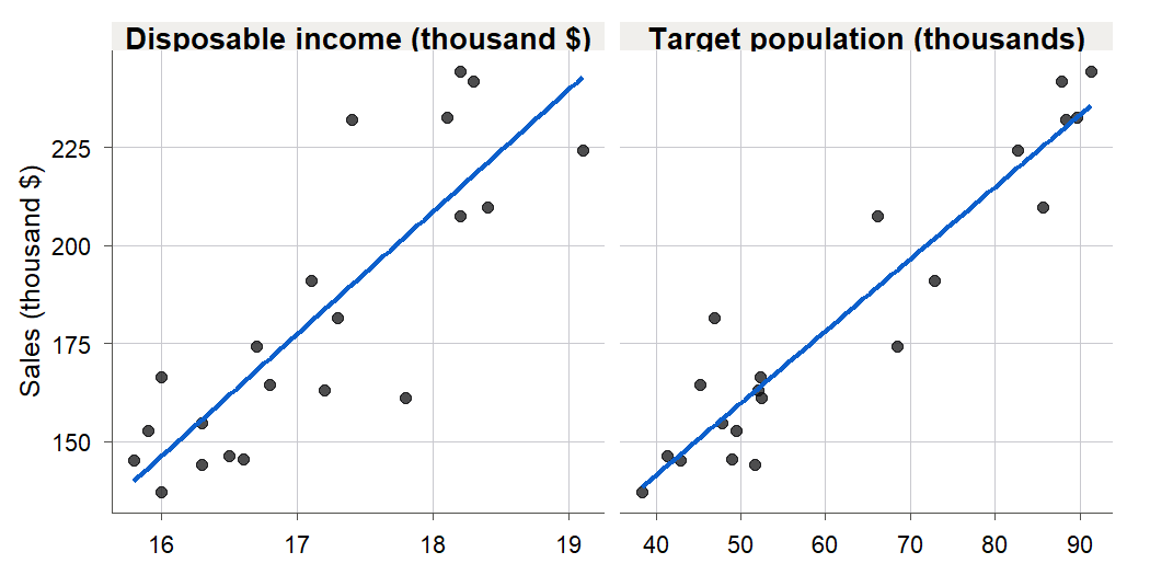
Figure 1:Dwaine Studios sales rise with both the young-population count and disposable income when each is viewed alone. Multiple regression asks a harder question: how much does each predictor add once the other is already in the model?
Simple linear regression, from Chapters 2 and 3, handles one predictor. Real questions almost always come with several. We could try to rebuild the whole theory predictor by predictor, but that path gets ugly fast: two predictors, then three, each with its own normal equations and variance formulas. Instead we do what 6. Matrix algebra for regression set up. We write the model once, in matrix form, so that one predictor or ten predictors look identical on the page. Every result from Chapter 2, the least-squares estimates, their unbiasedness, their variances, the Gauss-Markov optimality, the divisor, reappears here in a single clean form that works for any number of predictors at once. This chapter is where regression stops being a collection of special cases and becomes one general method.
This is the most abstract chapter in the course, and worth a word on how to read it. The geometry in 7.2 The geometry of least squares is the idea to hold onto: once you picture fitting as dropping a perpendicular from the data onto the space of possible fits, every proof that follows reduces to one of two facts about the hat matrix. Hold that picture and the algebra becomes bookkeeping.
7.1 The model and least squares in matrix form
Intuition
In Chapter 2 a single predictor gave one slope and one intercept. Add a second predictor and you have two slopes plus an intercept; the mean response is now a tilted plane instead of a line, as Figure 2 shows for Dwaine. With more predictors it is a flat sheet in a space you cannot picture. Writing separate symbols for every coefficient and separate sums for every normal equation would bury the idea under bookkeeping. The fix is to stack the observations into vectors and matrices and let one line of matrix algebra carry all the bookkeeping for us.
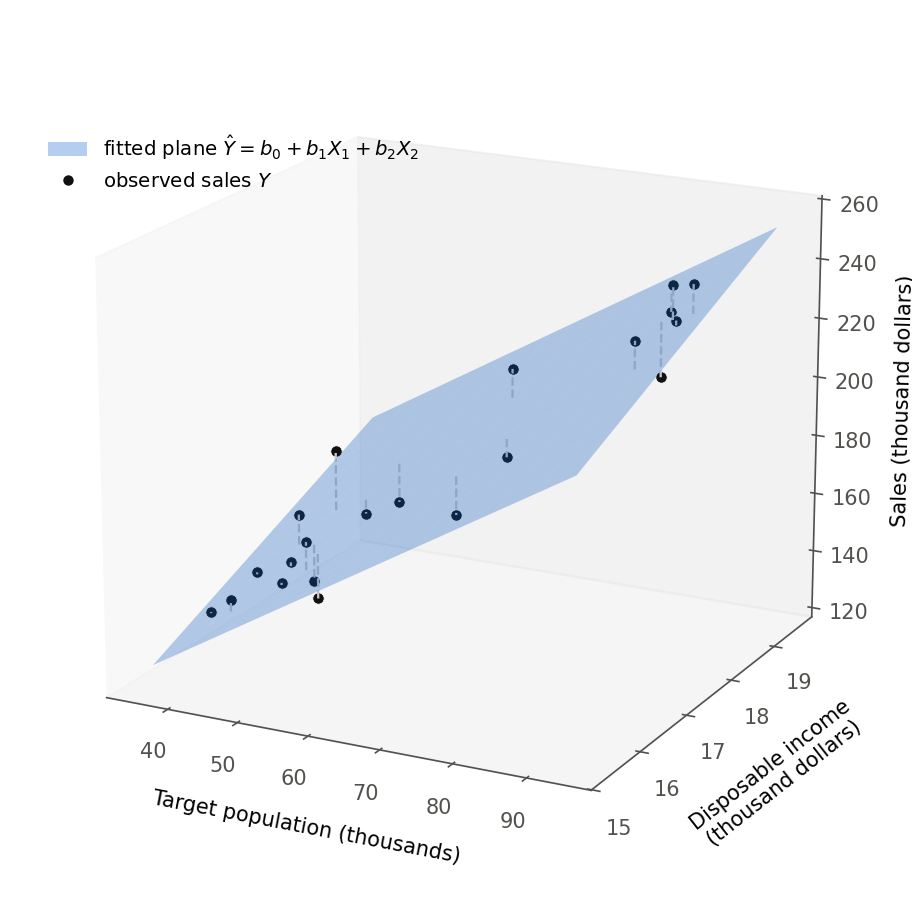
Figure 2:With one predictor the fit is a line; with two it is a tilted plane. Each city’s sales is a dark dot, the plane is the model’s guess, and each dashed stem is a residual. Multiple regression finds the plane whose stems are smallest in total squared length.
The systematic part of each observation is a weighted sum of that city’s predictor values, the same weights () reused for every city. Stacking the cities vertically turns “the same weights applied to every row” into a single matrix-times-vector product. Figure 3 shows the four objects and their shapes.
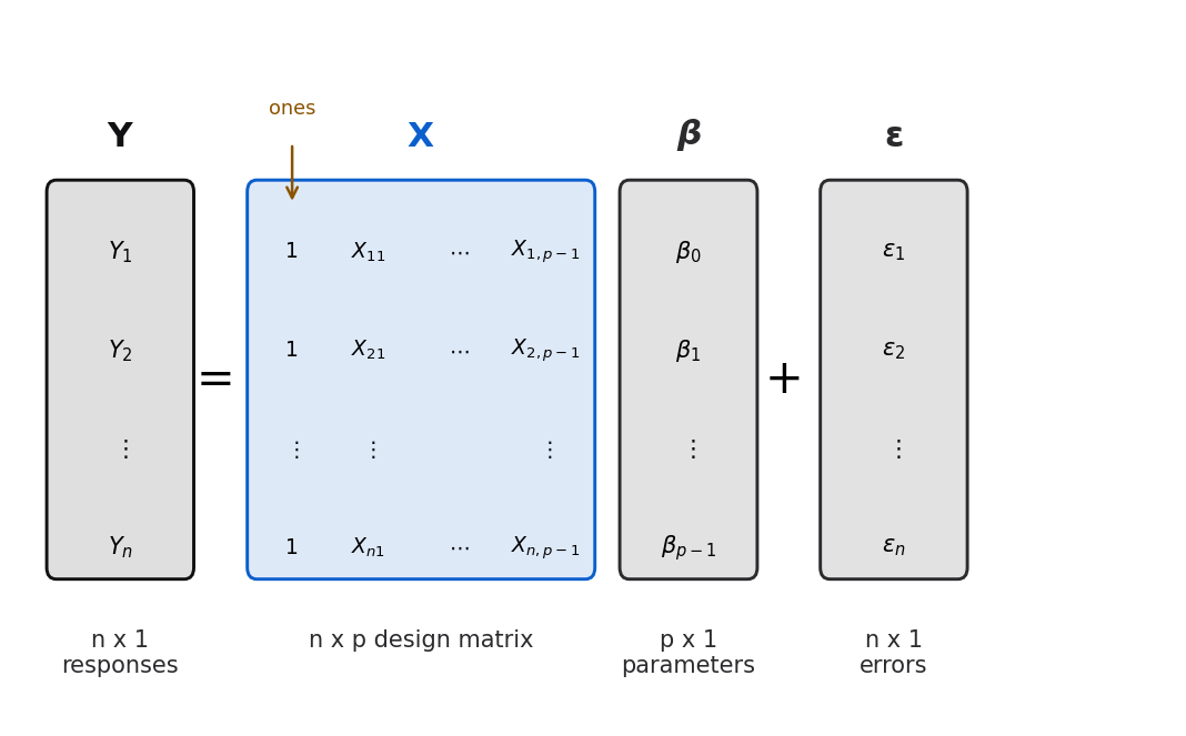
Figure 3:The general linear model as stacked arrays. The design matrix X carries a leading column of ones so that the intercept beta-0 is handled exactly like any other coefficient.
Formula
The general linear model (Definition 7.1) collects all observations into one matrix equation.
In words: each observation’s response equals a weighted sum of that observation’s predictor values plus a random error, and the same weights are reused for every row. The four objects are:
is the vector of responses, one entry per observation.
is the design matrix (Definition 7.2). Its first column is all ones (for the intercept); each remaining column holds one predictor’s values. Row is city ’s data.
is the vector of unknown parameters .
is the vector of random errors.
is the number of parameters, counting the intercept; with predictors, . Here and .
The error assumptions of Chapter 2 become two compact statements about the whole vector at once:
In words: every error averages to zero, and the covariance matrix is times the identity. That one symbol packs both assumptions at once: each error has the same variance (down the diagonal), and distinct errors are uncorrelated (off the diagonal). Because and are fixed, and as well. We assume throughout that has full column rank : no predictor is a copy of another, or an exact linear combination of the others. That is exactly what makes invertible (6.4 The inverse and the normal equations).
To fit the model we reuse the least-squares idea from 2.2 Least squares from first principles: pick the coefficient vector that makes the fitted values closest to the data in total squared error. Writing a candidate vector as , the sum of squared errors is
where is row of . In words: is the squared length of the residual vector, the same quantity Chapter 2 minimized, now written as one dot product. The minimizer is the least-squares estimator (Theorem 7.3)
In words: gather the cross-products of the predictors () and of the predictors with the response (), and multiply by the inverse of the first. We derive this next, then check it on Dwaine.
Derivation by calculus
Proof. Expand using the transpose rules of 6.2 Transpose and matrix multiplication. Since is a scalar, it equals its own transpose , so the two middle terms combine:
We minimize by taking the gradient with respect to and setting it to zero. The gradient is just the vector of partial derivatives, one per entry of , and setting it to zero finds the bottom of the bowl. Two vector-derivative rules do the work: for a constant vector , ; and for a symmetric matrix , . These are the vector twins of the scalar rules and you already know. The matrix is symmetric, so
Setting the gradient to zero and dividing by 2 gives the normal equations (Definition 7.4)
Because has full column rank, is invertible (6.4 The inverse and the normal equations), so we may multiply on the left by :
This stationary point is the global minimum, not a saddle or maximum, because the matrix of second derivatives of is , which is positive definite; a quadratic with a positive-definite Hessian is strictly convex and has a single lowest point.
These are the same normal equations as Chapter 2, now stated once for any number of predictors. In 2.2 Least squares from first principles the two scalar normal equations were and ; the single matrix equation contains both of those and one more for each extra predictor, as we will see in 7.7 Simple regression as a special case.
R
Chapter 6 built and for Dwaine by hand. Here we let the computer form them and solve.
dwaine <- read.csv("data/dwaine.csv")
head(dwaine, 3)
X <- cbind(1, dwaine$targtpop, dwaine$dispoinc)
Y <- dwaine$sales
dim(X)
targtpop dispoinc sales
1 68.5 16.7 174.4
2 45.2 16.8 164.4
3 91.3 18.2 244.2
[1] 21 37.2 The geometry of least squares
Intuition
The calculus derivation finds the answer but hides why it is the answer. There is a picture that makes least squares obvious, and it is worth carrying for the rest of the course. Think of the response as a single arrow (a point) in -dimensional space, one axis per observation. As the coefficient vector ranges over all possible values, the fitted vector traces out a flat subspace: every linear combination of the columns of . This subspace is the column space of (Definition 7.5), and it holds every prediction the model can possibly make.
The data point almost never sits exactly in that subspace, because real data has noise. So the fitting problem is: which point in the column space is closest to ? The closest point on a flat surface to an outside point is the foot of the perpendicular dropped from the point to the surface. That foot is , and the perpendicular segment is the residual vector . Figure 4 draws exactly this for the smallest case that fits on a page, three observations and two columns.
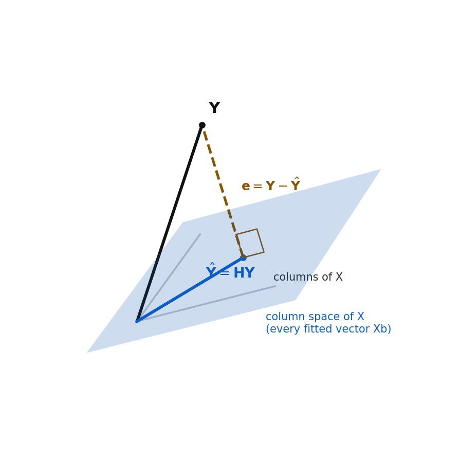
Figure 4:Least squares as projection. The fitted vector Y-hat is the point of the column space closest to Y, reached by dropping a perpendicular; the residual e is that perpendicular, meeting the column space at a right angle.
Formula
The geometric condition is that the residual is orthogonal to every column of :
In words: each column of , dotted with the residual vector, gives zero, so the residual points in a direction the model cannot represent. Expanding gives back the normal equations , so the geometry and the calculus lead to the identical solution.
Derivation by projection
Derivation (least squares as orthogonal projection). Let solve the normal equations, so with . Take any other candidate coefficient vector , with fitted vector . Split the gap from to that candidate by routing through :
The second piece lives in the column space. Its squared length adds without a cross term, because the cross term vanishes by orthogonality:
Therefore, by the Pythagorean theorem in dimensions,
with equality only when , that is . Since has full column rank, this forces . So the normal-equations solution gives the unique smallest sum of squared errors, and is the closest point of the column space to .
This is the same algebraic identity as the Chapter 2 proof in 2.2 Least squares from first principles, now read as geometry: the cross term vanishes there because and , which is precisely written out. The projection view (in 6.5 Idempotent and projection matrices) is the one to remember, because diagnostics in Chapter 9 are all about which observations sit in awkward corners of the column space.
R and Python
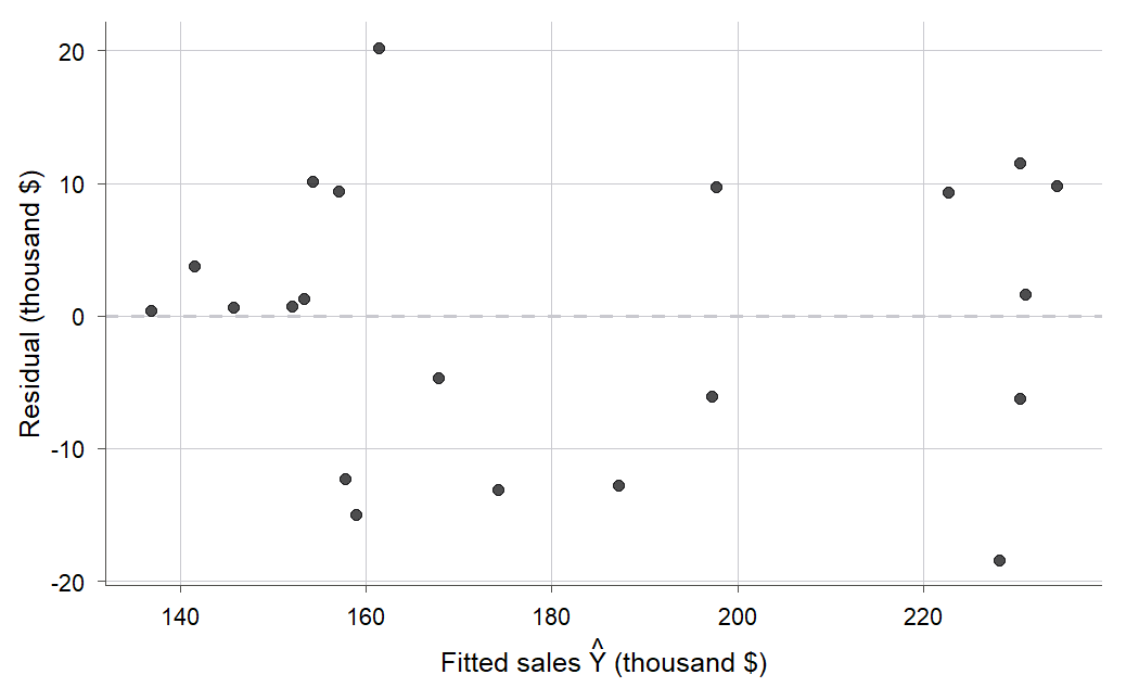
Figure 5:The Dwaine residuals against fitted values form a flat, patternless band around zero, the picture that supports the constant-variance and linearity assumptions. Chapter 9 turns this habit into a full diagnostic toolkit.
Orthogonality is easy to state and easy to doubt, so the simulation below hands you the data and invites you to break it.
Drag any of the seven cities anywhere you like. The slope and SSE respond, but both entries of X’e, and the Pythagoras gap SST minus SSR minus SSE, stay at zero.
7.3 The hat matrix
Intuition
Section 7.2 pictured the fit as a projection of onto the column space. That projection is carried out by a single matrix, and giving it a name pays off for the rest of the chapter. The fitted vector is a fixed linear function of the data: plug the formula for into and you get . The matrix sitting in front of turns the raw responses into fitted values, so it earns the name hat matrix (Definition 7.6): it puts the hat on . It is the single most useful matrix in the rest of the course. Its diagonal entries are the leverages that flag unusual predictor values (Chapter 9), and its algebra makes the variance results below fall out in a line.
Formula
The hat matrix and the fitted and residual vectors are
is and depends only on the predictors, not on .
: each fitted value is a fixed weighted average of all the responses, with weights read off a row of .
: the residual is what is left after projecting, so is itself a projection, onto the space perpendicular to the columns of .
Figure 7 shows the Toluca hat matrix as a grid of weights; the diagonal entries, outlined, are the leverages .
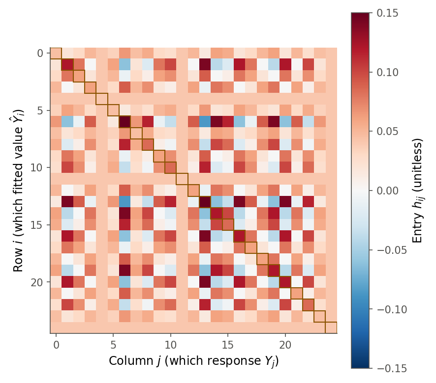
Figure 7:The Toluca hat matrix H turns responses into fitted values. Reading across row i gives the weights that build the i-th fitted value; the outlined gold diagonal entries are the leverage values that Chapter 9 uses to find unusual observations.
Derivation (properties of H)
Proof. Write , which is symmetric because is (the inverse of a symmetric matrix is symmetric, by 6.4 The inverse and the normal equations).
Symmetric. Using from 6.2 Transpose and matrix multiplication,
Idempotent. Projecting twice equals projecting once. The middle cancels its inverse:
Figure 8 shows why: once has landed a vector in the column space, projecting again cannot move it.
Trace . The trace of a matrix is the sum of its diagonal entries. Use the cyclic property of the trace, (a standard identity: both sides equal ), to slide around:
Consequently is also symmetric and idempotent, with . That trace is the degrees of freedom for error, and it is the reason the divisor in the variance estimate is , proved in 7.5 Estimating the error variance.
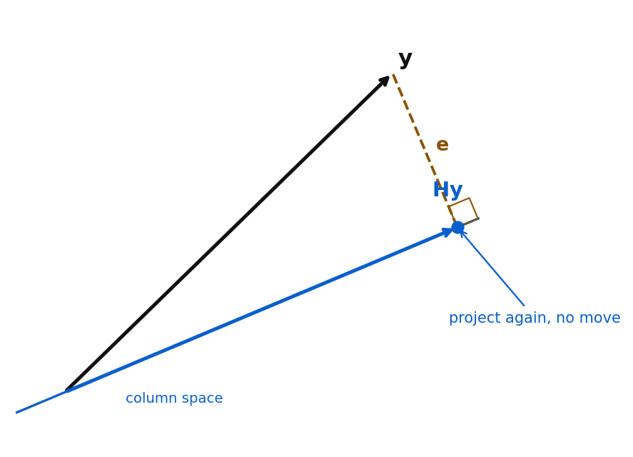
Figure 8:Why H is idempotent. Projecting the vector y onto the column space lands it at Hy inside that space; projecting a second time leaves it exactly where it is, so HH equals H.
R and Python
The claim that depends only on the predictors sounds like a technicality until you try to move it with the response, which is what the next simulation asks you to do.
Drag a city straight up and the leverages do not move at all; drag it sideways and they jump immediately, while the trace of H stays pinned at p.
7.4 The sampling distribution of b
Intuition
The vector came from one sample of 21 cities. A different 21 cities would give a slightly different , so is random, with a mean and a covariance across the samples we could have drawn. Two questions repeat from Chapter 2, now for a whole vector: is right on average, and how much does it vary? The answers are clean because is a fixed matrix times , and 6.7 Random vectors, expectation, and covariance matrices tells us exactly how means and covariances pass through a linear map.
Formula
The least-squares vector is unbiased with a covariance matrix built from :
In words: on average hits the true coefficient vector, and its covariance matrix is times the inverse cross-product matrix. The diagonal entries are the variances of the individual coefficients; the off-diagonal entries are the covariances between them, which is why two coefficients can be correlated (the tilted cloud in Figure 10). Replacing by its estimate gives the estimated covariance matrix , whose diagonal square roots are the standard errors software prints.
Derivation (mean and covariance of b)
Proof. Write with the fixed matrix . For a fixed matrix times a random vector, 6.7 Random vectors, expectation, and covariance matrices gives and .
Mean. Since ,
Covariance. Since ,
where the middle cancels one inverse and the symmetry of handles the transpose.
If we add the normality assumption , then is multivariate normal, and a fixed linear map of a multivariate normal is again multivariate normal (6.8 The multivariate normal, in brief). So
In words: under normal errors each coefficient is normally distributed around its true value, and this is what powers the tests and confidence intervals of Chapter 8. Figure 10 confirms the covariance by simulation: refitting many datasets scatters the two Dwaine slopes into a tilted ellipse that matches .
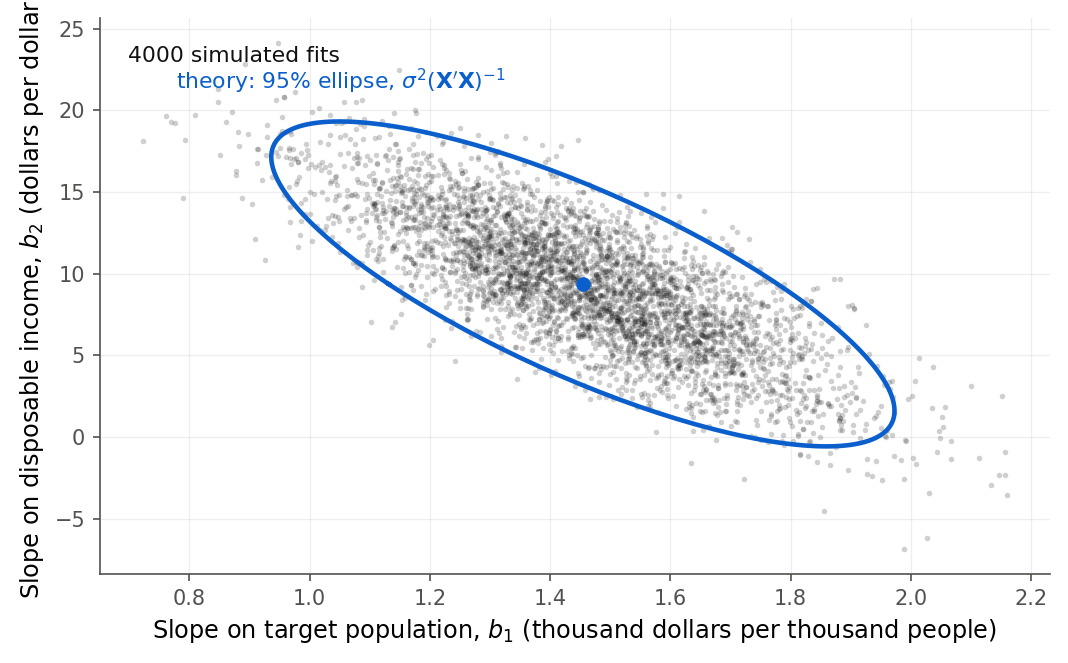
Figure 10:Simulating 4000 refits scatters the two Dwaine slope estimates into a tilted ellipse. The downward tilt is a negative covariance: the two slope estimates trade off, because the predictors are correlated. The blue theoretical ellipse from sigma-squared times the inverse cross-product matrix matches the simulated cloud.
R and Python
The covariance formula is a prediction about data you have not collected, so the simulation below collects it for you a thousand times and checks.
Each refit uses the same 21 cities with fresh errors. Press Draw 1000 and the spread of the b1 pile matches the standard error that the matrix formula predicted in advance.
7.5 Estimating the error variance
Intuition
The coefficients describe the plane; the model still has one more unknown, the error variance , which sets how far the data scatter off the plane. As in Chapter 2 we estimate it from the residuals, but now we must find the right divisor for a model with parameters instead of 2. The answer is , and the reason is the trace we computed in 7.3 The hat matrix: fitting coefficients uses up directions of the data, leaving directions for the residual to live in. Figure 12 keeps the bookkeeping in view: the directions of the data split into a fit part and a residual part, and we average the squared residual over its own directions, not all .
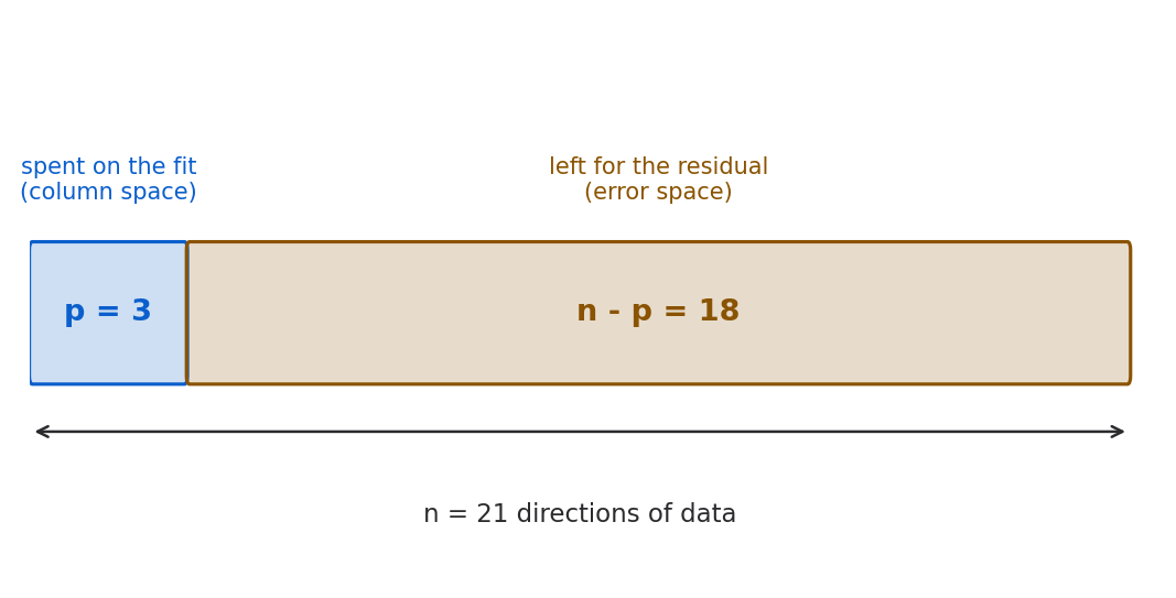
Figure 12:The n directions of the data split into p directions spent fitting the plane and n minus p left for the residual. Dividing SSE by n minus p, not by n, averages over exactly the directions the residual is free to fill, which is what makes MSE unbiased.
Formula
The error sum of squares and the estimator of are
is the squared length of the residual vector, the variation the model did not explain.
divides by its degrees of freedom , and estimates .
is the estimated error standard deviation, in the units of .
Derivation (why the divisor is n - p)
We need one fact about the expected value of a quadratic form. It is provable at our level, so we prove it, then apply it.
Lemma (expectation of a quadratic form). For any random vector with mean and covariance , and any fixed symmetric matrix ,
Proof. The scalar equals its own trace, and the trace is cyclic, so . Taking expectations and using (6.7 Random vectors, expectation, and covariance matrices),
since is a scalar.
Proof of Theorem 7.9. Apply the lemma with , , and . The two pieces are:
Trace piece. , using the trace from 7.3 The hat matrix.
Mean piece. The mean term vanishes, because (the hat matrix leaves the columns of unchanged, since they already lie in the column space). Therefore
Combining, , so
The divisor , and no other, makes unbiased.
This is the Chapter 2 result generalized: there gave the divisor ; here any model divides by minus the number of parameters. Figure 13 shows what goes wrong with the naive divisor : dividing by instead of biases the estimate low, and the gap is largest when is a big fraction of .
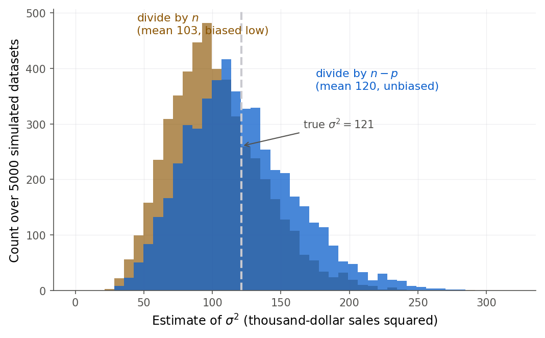
Figure 13:Dividing SSE by n - p (blue) centers the variance estimate on the truth; dividing by n (gold) pulls it systematically low. The bias is the price of estimating p coefficients before measuring the residuals.
R and Python
We can also read off how well the plane fits overall. The total variation splits into the part the model explains and the part it does not, and reports the explained fraction, exactly as in 3.6 The analysis of variance approach but now for many predictors.
SSTO <- sum((Y - mean(Y))^2)
SSR <- SSTO - SSE
c(SSTO = round(SSTO, 2), SSR = round(SSR, 2), SSE = round(SSE, 2),
  R2 = round(1 - SSE / SSTO, 4))
SSTO SSR SSE R2
26196.2100 24015.2800 2180.9300 0.9167SSTO = np.sum((Y - Y.mean()) ** 2)
SSR = SSTO - SSE
print(round(SSTO, 2), round(SSR, 2), round(SSE, 2), round(1 - SSE / SSTO, 4))26196.21 24015.28 2180.93 0.9167The two predictors together explain about of the variation in Dwaine sales. Chapter 8 unpacks this number, warns about how it can only rise when predictors are added, and builds the general linear test on top of the we just computed (8.3 Extra sums of squares).
7.6 The Gauss-Markov theorem
Intuition
We chose least squares because squared error is a natural penalty, and Chapter 2 rewarded that choice: in simple regression, no other linear unbiased estimator beats . The same reward holds for the full vector, and the matrix proof is barely longer than the scalar one. The claim is that any competitor built as a fixed linear combination of the responses, and required to be right on average, must have a covariance matrix at least as large as 's. No normality is needed; the mean-zero, constant-variance, uncorrelated error assumptions are enough. Figure 14 shows the payoff on Toluca: least squares and a competing unbiased estimator are both centered on the truth, but least squares scatters far less.
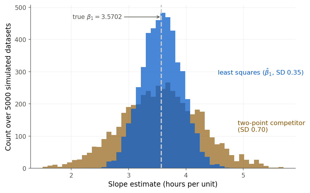
Figure 14:Both the least-squares slope (blue, narrow) and a two-point competitor (gold, wide) are unbiased, centered on the true slope. Least squares has the smaller spread, exactly what the Gauss-Markov theorem guarantees.
Formula
Derivation (b is BLUE)
Proof. Let be any linear estimator with a fixed matrix . Its mean is . For to be unbiased for for every possible , we need
Write , defining as the difference from the least-squares matrix. The unbiasedness condition becomes
Now compute the covariance. Since , . Expand with . The two cross terms vanish because (and its transpose ):
What survives is
Therefore
For any fixed , the variance of the scalar is
The added term is a squared length, so every linear unbiased competitor has variance at least that of , with equality only when ; taking to range over the coordinate vectors forces , that is, the competitor is itself. Least squares is BLUE.
Setting and recovers the Chapter 2 statement that is BLUE (2.5 Sampling behavior and the Gauss-Markov theorem); the matrix proof did every coefficient, and every linear combination of coefficients, at once.
7.7 Simple regression as a special case
Intuition
Everything in Chapters 2 and 3 should drop out of the matrix formulas when there is one predictor, and it does. Seeing it happen once turns the general formulas from abstractions into trusted tools: the same machine that fit Dwaine’s plane fits Toluca’s line, and returns the exact numbers you already know. Figure 15 is the whole idea in one picture: one formula, two jobs.
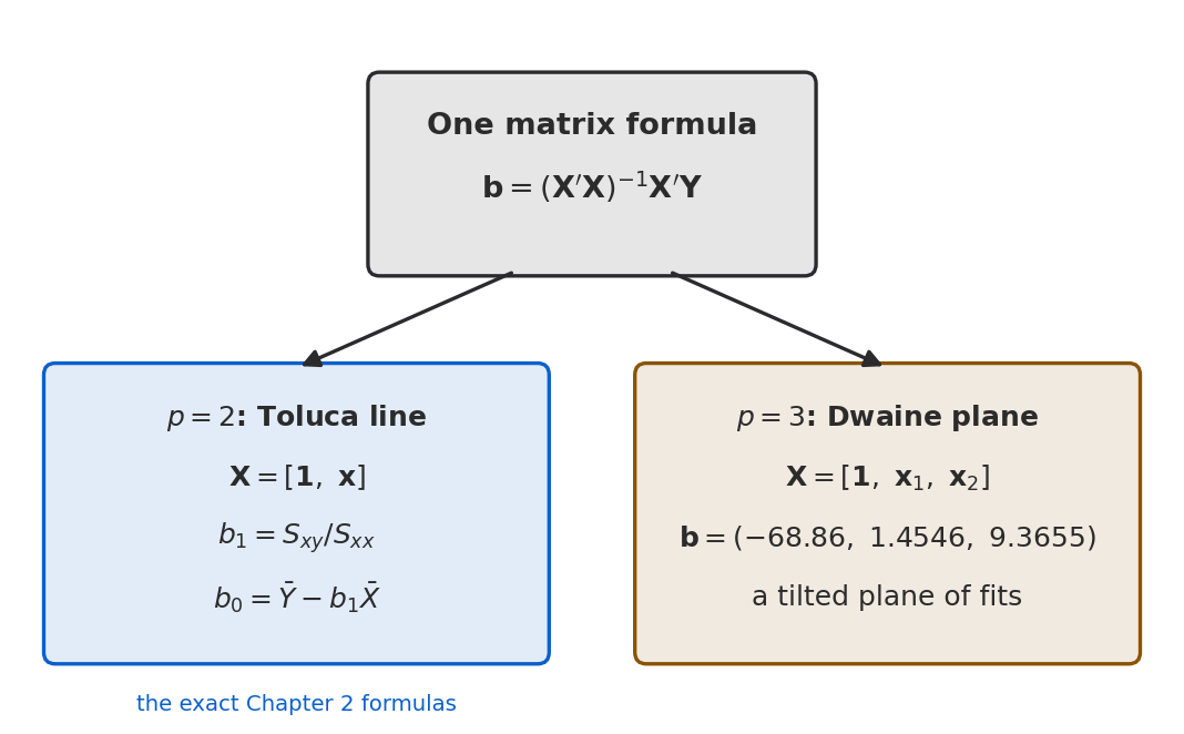
Figure 15:One matrix formula does two jobs. Set p equals 2 and it collapses into the exact Chapter 2 scalar formulas for the Toluca line; set p equals 3 and it fits the Dwaine plane. The general model does not replace simple regression, it contains it.
Derivation (matrix formulas reduce to Chapter 2)
Derivation (the case). With one predictor, the design matrix is , so
where and are the Chapter 2 sums of squares and cross-products, and are the sample means. The inverse of a matrix divides by its determinant (6.4 The inverse and the normal equations),
Multiplying by and simplifying (each entry collapses using and the definitions of ) gives
which are exactly the Chapter 2 estimators and . The covariance matrix reduces the same way: the bottom-right entry of is , matching , and the top-left entry is , matching from 2.5 Sampling behavior and the Gauss-Markov theorem.
Example 7.5 already confirmed this numerically: the matrix pipeline returned Toluca’s , , and standard errors 26.1774 and 0.3470, the same figures Chapter 2 produced from the scalar formulas. The general linear model does not replace simple regression; it contains it.
7.8 Chapter summary
This chapter turned Chapter 6’s matrix arithmetic into a full multiple regression. One equation, , carries any number of predictors. Least squares projects onto the column space of , giving by calculus and by geometry alike. The hat matrix packages that projection, and its two properties, being a projection (symmetric and idempotent) with trace , drive the sampling distribution of , the divisor in , and the Gauss-Markov optimality. Every Chapter 2 formula returns as the special case.
Key results at a glance.
| Result | Statement or formula | Valid when |
|---|---|---|
| Least-squares estimator (Theorem 7.3) | minimizes | full column rank |
| Normal equations (Definition 7.4) | , equivalently | any least-squares fit |
| Hat matrix properties (Theorem 7.7) | symmetric, idempotent, , | full column rank |
| Mean and covariance of (Theorem 7.8) | , | , |
| Sampling distribution (Theorem 7.8) | errors also normal | |
| Unbiasedness of MSE (Theorem 7.9) | , so | |
| Gauss-Markov (Theorem 7.10) | is the best linear unbiased estimator of | , ; no normality needed |
| Coefficient of determination | (Dwaine 0.9167) | descriptive, any fit |
Key terms. general linear model, design matrix, normal equations, least-squares estimator, column space, hat matrix, idempotent matrix, full column rank, error degrees of freedom, best linear unbiased estimator (BLUE).
You should now be able to.
Write any linear regression as and identify the design matrix, coefficient vector, and error vector.
Derive two ways: by calculus and by orthogonal projection.
Interpret least squares geometrically as projecting onto the column space of , with the residual perpendicular to it.
Prove that the hat matrix is symmetric and idempotent with trace , and use it to write fitted values and residuals.
Derive the mean and covariance of and state its sampling distribution under normal errors.
Prove that is unbiased for using the trace of .
State and prove the Gauss-Markov theorem in matrix form: is the best linear unbiased estimator.
Recover every simple-regression formula from Chapter 2 as the special case .
Where this fits. This chapter is the general engine for the FIT stage of the course workflow (The modeling workflow): it estimates the coefficients and the error variance for a model of any size, replacing the predictor-by-predictor algebra of Chapters 2 and 3 with one formula that a computer can run for ten predictors as easily as one. It also arms the CHECK stage, because the hat matrix is the object Chapter 9 (9. Model diagnostics) turns into the leverage values and influence measures, and the USE stage, because is what Chapter 8 turns into tests and intervals. Chapter 8 takes the Dwaine fit built here, interprets each coefficient with care, and develops the extra-sums-of-squares and general-linear-test machinery (8.3 Extra sums of squares) that decides which predictors a model needs.
7.9 Frequently asked questions
Q1. Why does the design matrix need a column of ones? The column of ones lets the intercept be handled like any other coefficient: its “predictor value” is 1 for every observation, so is the same baseline for every row. Without it the fitted plane would be forced through the origin. The first normal equation, coming from that column, is exactly .
Q2. What does full column rank mean, and what breaks without it? Full column rank means no predictor column is a linear combination of the others (including the ones column). If one is, say a predictor recorded in both meters and feet, then is singular and does not exist, so there is no unique : infinitely many coefficient vectors fit equally well. Software then drops a column or returns an error. Near-violations (highly correlated predictors) are multicollinearity, the subject of Chapter 12.
Q3. Is the hat matrix worth computing for real data? As a full matrix, usually not; software gets fitted values and residuals more cheaply. But its diagonal entries , the leverage values, are computed and used constantly in diagnostics, and its algebra (symmetric, idempotent, trace ) is what makes the theory work. Think of as a proof tool and a source of the leverages, not a thing you print.
Q4. Why is the divisor and not or ? Each parameter you estimate uses one degree of freedom before the residuals are measured. A sample variance estimates one quantity (the mean) and divides by ; a regression with parameters divides by . The trace derivation in 7.5 Estimating the error variance shows exactly, so is the unique divisor making unbiased. Dividing by (the maximum-likelihood choice) is biased low.
Q5. Do I need normal errors for any of this? No, for most of it. The estimator , its unbiasedness, its covariance , the unbiasedness of , and the Gauss-Markov optimality all hold with only mean-zero, constant-variance, uncorrelated errors. Normality is an extra assumption, used to get the exact multivariate normal sampling distribution of and the and tests of Chapter 8.
Q6. The Dwaine coefficients from the matrix formula and from lm matched exactly.
Is that always guaranteed? Yes, up to tiny floating-point differences. Both compute
the same ; lm and statsmodels
use a more numerically stable routine (a QR or SVD decomposition) instead of forming
the inverse explicitly, which matters only for badly conditioned designs. For
well-behaved data like these, every printed digit agrees.
Q7. Why are the two Dwaine slope estimates negatively correlated in Figure 10? Because the two predictors are themselves positively correlated across cities. When a sample happens to make the population slope come out high, the fit compensates by making the income slope come out low to avoid double-counting the shared signal. That trade-off is exactly the off-diagonal entry of , and it is why you cannot read one coefficient’s uncertainty without the whole covariance matrix.
7.10 Practice problems
(A) Write the Dwaine model in the form , giving the dimensions of each of the four objects and describing the first column of .
(A) Explain in one sentence each what and represent, and why the normal equations use them.
(A) State the two error assumptions and in plain words, saying what the diagonal and the off-diagonal of each encode.
(A) In the projection picture, what is the column space of , where does sit, and in what direction does the residual point? Answer without formulas.
(A) Give the three properties of the hat matrix proved in this chapter and say what each one means geometrically.
(A) Why is the divisor in equal to ? Answer by naming what the number counts and what counts.
(A) A colleague says “with normality the least-squares estimator is BLUE; without it, it is not.” Correct the statement, naming exactly which assumptions the Gauss-Markov theorem uses.
(A) Explain why (an matrix) cannot replace in the normal equations.
(B) Starting from , expand it, take the gradient, and derive the normal equations and (Theorem 7.3). Justify why the stationary point is a minimum.
(B) Prove the projection identity for any , showing the cross term vanishes, and conclude that uniquely minimizes SSE.
(B) Prove that is symmetric and idempotent (Theorem 7.7). Then prove is symmetric and idempotent as well.
(B) Prove using the cyclic property of the trace, and deduce .
(B) Show and use it to prove . Explain in words why the hat matrix leaves the columns of unchanged.
(B) Derive and (Theorem 7.8), naming the random-vector facts you use at each step. Then, adding the assumption , state the full sampling distribution of and explain why the mean and covariance did not need normality but this distributional statement does.
(B) Prove the quadratic-form lemma , then use it to show (Theorem 7.9).
(B) State and prove the Gauss-Markov theorem in matrix form (Theorem 7.10). Where in the proof does the assumption enter, and where does full column rank enter?
(B) For the simple-regression design , compute , its determinant, and , and derive and from the matrix formula.
(B) Using the reduction in problem 17, derive and from .
(B) Show that under the model, using , , and . Why does this matter for diagnostics?
(B) Prove that adding a predictor (a new column to ) cannot increase , using the projection argument that enlarging the column space can only move closer to .
(C) Read
dwaine.csv, build and , and compute from in R or Python. Confirm your answer matcheslm/smf.ols.(C) For the Dwaine fit, compute the residual vector and verify numerically that (all three entries) and that .
(C) Build the Dwaine hat matrix and verify it is symmetric and idempotent and has trace 3. Then report the five largest diagonal entries and say what a large indicates about that city’s predictors.
(C) Compute , , and for Dwaine two ways: from the residual vector, and from
summary/.summary2(). Then compute and report the percentage by which it understates .(C) Compute the estimated covariance matrix for Dwaine, report the three standard errors, and confirm they match the built-in summary. Report the correlation between the two slope estimates from the off-diagonal entry.
(C) Refit Toluca through the matrix formulas and confirm , , , and the two standard errors, matching Chapter 2 to every digit.
(C) Write a simulation (seed
4210) that draws 2000 datasets from the fitted Dwaine model, refits each, and reports the mean of the 2000 estimates of each coefficient (checking unbiasedness) and the standard deviation of the target-population slope (checking ).(C) Regress Dwaine
salesontargtpopalone, then ontargtpopanddispoinctogether, and confirm numerically that addingdispoinclowers . Relate the drop to the projection argument in problem 20.
7.11 Exam practice
EP 7.1 (interpret output in context). A colleague fits the Dwaine model in R and reads off the coefficient table.
            Estimate Std. Error t value Pr(>|t|)
(Intercept) -68.8571    60.0170 -1.1473   0.2663
targtpop      1.4546     0.2118  6.8682   0.0000
dispoinc      9.3655     4.0640  2.3045   0.0333
Interpret the targtpop coefficient and its value in the context of studio sales,
being explicit about what is held fixed. Then evaluate the colleague’s conclusion:
“the intercept has , so it is not significantly different from zero, which
means the model is misspecified and we should drop the intercept.” Say whether the
conclusion is right and why.
Model answer
Holding disposable income fixed, each additional thousand young residents in a city is associated with about 1.4546 thousand dollars, roughly $1{,}455, of additional predicted annual sales. The value of 6.87 is the estimate divided by its standard error (); it is far from zero and its -value is essentially zero, so the target-population slope is clearly distinguishable from zero at any usual level, and target population carries real predictive signal once income is already in the model.
The colleague’s conclusion is wrong on both counts. The intercept’s insignificance means only that the data cannot pin down the fitted plane’s height at the point where both predictors equal zero, which is far outside the range of any real city (populations near 62 thousand and incomes near 17 thousand dollars in these data), so a loose intercept there is expected and harmless. An insignificant intercept is not evidence of misspecification, and dropping the intercept is a strong, usually wrong, modeling choice: it forces the fitted plane through the origin, distorts every slope, and breaks the identity that the column of ones guarantees. Keep the intercept.
A weak answer reports the slope as a raw number without the “holding income fixed” comparison or the units, and treats the intercept’s large -value as a defect to fix rather than a statement about an extrapolated region no city occupies.
EP 7.2 (explain why, and what would change if). Explain in full sentences why the divisor in is and not . Then answer a “what would change if”: suppose an analyst kept adding predictors to the Dwaine data until the model had parameters, one for every observation. Describe what happens to , to the divisor, and to , and explain why a fit with is a warning rather than a success.
Model answer
The divisor is because fitting coefficients uses up of the independent directions in the data before the residuals are measured. Formally, and , so ; dividing by , and no other number, makes an unbiased estimator of . Dividing by would systematically underestimate the error variance.
If , the column space of fills the whole 21-dimensional response space, so the projection equals exactly and every residual is zero, giving . The divisor , so is undefined: there are no error degrees of freedom left. A zero does not mean the model is perfect; it means the model has enough parameters to interpolate the data exactly, so it has learned the noise along with the signal and can say nothing about or about a new city. Perfect in-sample fit with zero degrees of freedom is the signature of overfitting.
A weak answer says “ adjusts for the parameters” without connecting it to unbiasedness or the trace, and treats as a good outcome instead of recognizing that zero error degrees of freedom leave nothing to estimate the variance with.
EP 7.3 (a student claims X, evaluate). A student writes: “Adding a predictor can never increase , and it always raises . So the best strategy is to keep adding predictors until is as close to 1 as possible.” Using the projection picture of least squares, evaluate the two factual claims and the strategy they support.
Model answer
The two factual claims are true. Adding a column to enlarges its column space, and projecting onto a larger subspace can only bring the foot of the perpendicular closer to , never farther, so cannot rise; the old fit is still available as a special case where the new coefficient is zero. Because and is fixed, a non-increasing means a non-decreasing .
The strategy, however, is wrong. Since rises even for predictors that are pure noise, a high bought by piling on predictors is not evidence of a good model; in the limit the fit interpolates the data with and while explaining nothing out of sample. Each added predictor also spends a degree of freedom, shrinking and inflating the variances of the coefficients, especially when the new predictor is correlated with those already present. The right question is not whether dropped but whether it dropped by more than noise would predict, which is exactly what the general linear test of Chapter 8 measures.
A weak answer either wrongly disputes the two true facts or accepts the strategy, missing that a guaranteed rise in carries no information about whether a predictor belongs in the model.
EP 7.4 (interpret computed output in context). The leverage values are the diagonal entries of the hat matrix for the Dwaine fit. The six largest, and a check on their sum, are below.
row 20  targtpop=  82.7  dispoinc= 19.1  h_ii=0.2788
row 13  targtpop=  88.4  dispoinc= 17.4  h_ii=0.2390
row 15  targtpop=  52.5  dispoinc= 17.8  h_ii=0.2095
row  3  targtpop=  91.3  dispoinc= 18.2  h_ii=0.1737
row  5  targtpop=  46.9  dispoinc= 17.3  h_ii=0.1620
row 19  targtpop=  89.6  dispoinc= 18.1  h_ii=0.1611
sum(h_ii) = 3.0000     mean(targtpop)=62.02  mean(dispoinc)=17.14
Explain what a large says about a city, and interpret why row 20 has the largest leverage value even though its target population (82.7) is not the largest in the data. Then explain why the leverage values sum to exactly 3, and use the rule-of-thumb cutoff to say whether any Dwaine city should be called a high-leverage point.
Model answer
A large means the city sits far from the center of the predictor cloud, so its predictor values are unusual and its own response pulls its fitted value strongly toward itself. Row 20 has the largest leverage value not because of any single coordinate but because of the combination: its disposable income 19.1 is the highest in the data, well above the mean of 17.14, and its target population 82.7 is also well above the mean of 62.02, so it sits in a far corner of the two-dimensional predictor space. The leverage value measures distance from the joint center, so a city can have a higher leverage value than one with a larger population alone if it is more extreme on both predictors together.
The leverage values sum to 3 because , proved in 7.3 The hat matrix: the trace of the projection matrix counts the parameters, so the total of the leverage values the fit distributes across cities is fixed at regardless of the data. Against the cutoff , the largest leverage value (0.2788) falls just below it, so by this rule of thumb no Dwaine city is flagged as a high-leverage point; the design is fairly balanced, with no city dominating the predictor space.
A weak answer reads the leverage value off target population alone, misses that it measures joint distance from the center of both predictors, and cannot explain the sum-to- property as the trace of .
EP 7.5 (what would change if). An analyst re-expresses target population in hundreds
of people instead of thousands, multiplying every targtpop value by 10, and refits.
The two coefficient tables are below.
original                              rescaled
             Estimate Std. Error       Estimate Std. Error
(Intercept)  -68.8571    60.0170       -68.8571    60.0170
targtpop       1.4546     0.2118        0.1455     0.0212
dispoinc       9.3655     4.0640        9.3655     4.0640
original  MSE=121.16  R2=0.9167     rescaled  MSE=121.16  R2=0.9167
Explain, in full sentences and with reference to the model algebra, why the target- population coefficient and its standard error both divide by 10 while its value, the fitted values, , and are all unchanged. What does this tell you about reading the size of a coefficient as a measure of a predictor’s importance?
Model answer
Rescaling a predictor by a factor of 10 replaces its column by . For the fitted plane to make the same predictions, the coefficient on that column must divide by 10, since : the product that enters is unchanged, so the fitted values, the residuals, , , and are all identical to the original fit. The standard error divides by 10 for the same reason the estimate does, because it is measured in the coefficient’s own units (dollars per hundred people instead of dollars per thousand people), so the ratio is dimensionless and does not move; the evidence that the slope differs from zero is exactly as strong as before.
The lesson is that the raw magnitude of a coefficient is not a measure of a predictor’s importance, because you can make a coefficient ten times larger or smaller just by changing the units of its predictor, with no change to the fit or to the strength of the evidence. To compare importance you must look at scale-free quantities such as the value, or standardize the predictors first.
A weak answer states that the numbers change without tying the factor of 10 to the product staying fixed, and fails to draw the conclusion that coefficient size, being unit-dependent, cannot rank predictors by importance.
7.12 Chapter game
Resumen del capítulo (en español)
Este capítulo presenta el modelo lineal general (general linear model) , que escribe cualquier regresión, con uno o con muchos predictores, en una sola forma matricial. La matriz de diseño (design matrix) tiene una primera columna de unos para el intercepto y una columna por cada predictor; reúne los parámetros y los errores, con y .
El estimador de mínimos cuadrados (least squares) es , obtenido de dos maneras: por cálculo, derivando las ecuaciones normales (normal equations) ; y por proyección ortogonal (orthogonal projection), donde es el punto del espacio de columnas de más cercano a y el residuo es perpendicular a ese espacio. Para Dwaine Studios, .
La matriz sombrero (hat matrix) cumple y es simétrica e idempotente con traza . De ahí sale que , el divisor correcto para estimar la varianza: es insesgado (unbiased), lo cual se prueba con un argumento de traza. Para Dwaine, y .
El vector tiene media y covarianza ; bajo errores normales sigue una distribución normal multivariante. El teorema de Gauss-Markov (Gauss-Markov theorem) demuestra que es el mejor estimador lineal insesgado, sin necesitar normalidad. Finalmente, la regresión simple del Capítulo 2 aparece como el caso : las fórmulas matriciales reproducen , y de la Toluca Company, dígito por dígito.