In 2.2 Least squares from first principles we fit a line to the Toluca Company’s 25 production runs and got a slope of hours per unit of lot size. The engineers were pleased, and then they asked the questions any careful person asks about a number: how sure are you? A different 25 runs would have given a slightly different slope. Could the true slope really be zero, meaning lot size does not affect hours at all and we are fooling ourselves? And the practical one, the reason they collected the data: if we schedule a new run of 100 units next week, how many hours should we budget, and how far off might that be?
Chapter 2 gave point estimates: single best guesses for the intercept, slope, and error variance. A point estimate with no measure of its uncertainty is half an answer. This chapter supplies the other half. We attach margins of error to the slope and intercept, test whether the slope is really different from zero, and, most importantly for planning, build two very different intervals around a prediction. One says where the average run of a given size lands. The other says where a single new run lands. Figure 1 shows both drawn around the Toluca line, and the gap between them is the single most useful idea in the chapter.
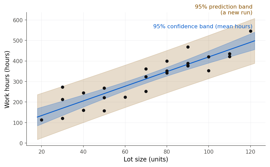
Figure 1:The inner (blue) band is a 95% confidence band for the mean hours at each lot size; the outer (yellow) band is a 95% prediction band for a single new run. The prediction band must cover one run’s own random scatter, so it is far wider. Confusing the two is the most common and most expensive mistake in applied regression.
Everything here rests on one added assumption that Chapter 2 introduced but did not yet use for inference: the errors are normally distributed (2.6 Maximum likelihood under normal errors). With that assumption the sampling distributions sketched in 2.5 Sampling behavior and the Gauss-Markov theorem become exact and distributions, and honest intervals and tests follow.
3.1 The sampling distributions of and 
Intuition
We already know from 2.5 Sampling behavior and the Gauss-Markov theorem that the slope estimate is unbiased, with variance , where is the spread of the predictor values about their mean . That tells us where centers and how much it spreads, but not the shape of its distribution. To build an interval we need the shape. The trick is that is a weighted sum of the responses, and a weighted sum of independent normal random variables is itself normal. So the moment we assume normal errors, is exactly normal, and we can standardize it the way intro statistics standardizes a sample mean.
There is one wrinkle. Standardizing needs the true error standard deviation , which we do not know. We replace it with the estimate . Swapping a known constant for a noisy estimate adds a little extra uncertainty, and that extra uncertainty is exactly what turns the normal distribution into a distribution. Figure 2 confirms this: standardize 5000 simulated slopes by their own estimated standard errors, and the pile matches a curve, with slightly heavier tails than the normal.
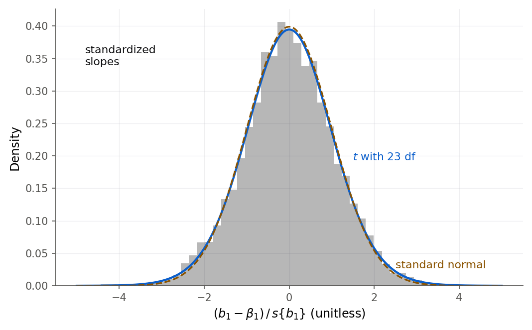
Figure 2:Five thousand slope estimates, each standardized by its own estimated standard error. The pile follows a t distribution with 23 degrees of freedom (red), whose tails are a touch heavier than the standard normal (dashed). Using s in place of sigma is what makes the reference distribution t rather than normal.
Formula
Under the normal error model with , the estimators are exactly normal:
In words: each estimator is centered on the parameter it estimates, with the variance we derived in Chapter 2, and now with a normal shape. To standardize either one we need the spread of the estimate. The estimated standard error of the slope (Definition 3.1) supplies it.
The estimated standard error is our best guess at how much bounces from one sample to the next. Standardizing with it gives a statistic, the result stated next.
In words: subtract the true value and divide by the estimated standard error, and the result follows a distribution with degrees of freedom. The degrees of freedom are because that is the divisor in , the two lost degrees paying for and (2.4 Estimating the error variance). This single result powers every interval and test in the rest of the chapter.
That last sentence is worth a picture. Almost everything ahead is one idea, the statistic above, pointed at a different estimate each time. Figure 3 is the map of the chapter on one page: keep it in mind and each new section becomes “the same move, new target.”
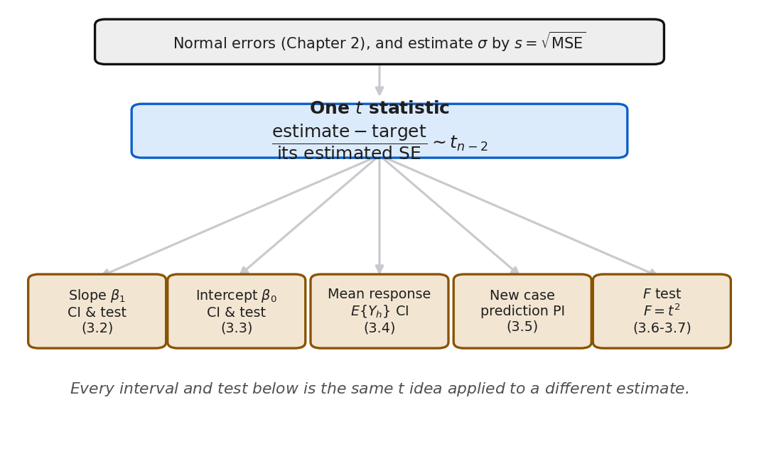
Figure 3:The whole chapter on one page. Take one estimate, subtract what it is trying to hit, divide by its estimated standard error, and read the answer off a t distribution. Every section ahead is that single move aimed at a new target.
Derivation
Derivation (the statistic for the slope). We assemble the result from three facts.
Normality. From 2.5 Sampling behavior and the Gauss-Markov theorem, with . Under the normal error model the are independent normal variables, and any linear combination of independent normals is normal. With the mean and variance already derived, . Dividing by the true standard deviation gives a standard normal:
A chi-square, independent of the slope. It can be shown that
and that this quantity is statistically independent of (indeed of the whole vector ). The clean proof uses the hat matrix and a theorem on quadratic forms in normal vectors; we give it in full in 7.3 The hat matrix, once we have the matrix tools. For now we take these two facts on faith, and note that the simulation in Figure 2 is a direct check that the end result is right.
Combine into a . A standard normal divided by the square root of an independent chi-square over its degrees of freedom is, by definition, a random variable:
The middle step just multiplies top and bottom out: the numerator is , and . The identical argument with the weights from 2.5 Sampling behavior and the Gauss-Markov theorem gives the statistic for .
The setup code below refits the Toluca model and recovers the standard errors we will use throughout.
toluca <- read.csv("data/toluca.csv")
fit <- lm(hours ~ lotsize, data = toluca)
n <- nrow(toluca)
x <- toluca$lotsize
y <- toluca$hours
Sxx <- sum((x - mean(x))^2)
MSE <- sum(residuals(fit)^2) / (n - 2)
round(c(n = n, Sxx = Sxx, MSE = MSE, s = sqrt(MSE),
        se_b1 = sqrt(MSE / Sxx)), 4)
n Sxx MSE s se_b1
25.0000 19800.0000 2383.7156 48.8233 0.3470 import numpy as np
import pandas as pd
import statsmodels.formula.api as smf
toluca = pd.read_csv("data/toluca.csv")
fit = smf.ols("hours ~ lotsize", data=toluca).fit()
n = len(toluca)
x = toluca["lotsize"].to_numpy()
y = toluca["hours"].to_numpy()
Sxx = np.sum((x - x.mean()) ** 2)
MSE = np.sum(fit.resid ** 2) / (n - 2)
print(round(MSE, 4), round(np.sqrt(MSE), 4), round(np.sqrt(MSE / Sxx), 4))2383.7156 48.8233 0.347The estimated standard error of the slope is hours per unit, the same number Chapter 2 computed from the variance formula. It is the yardstick for everything that follows.
3.2 Inference for the slope
Intuition
The slope is usually the number a study is about: does lot size affect hours, and by how much? Two questions come in a pair. A confidence interval (Definition 3.3) answers “how much?” by giving a range of plausible values for . A hypothesis test answers “is there any effect at all?” by asking whether zero is a plausible value. Both are built from the one statistic of 3.1 The sampling distributions of and , so they always agree: a 95% interval excludes zero exactly when the two-sided test rejects at the 5% level.
Formula
In words: take the estimate and reach out a multiplier’s worth of standard errors on each side. To test against , form the test statistic
and reject when , or equivalently when the two-sided p-value is below . In words: if the estimate sits many standard errors away from zero, zero is not credible. Nothing here is special to zero; to test for any value , put in place of the 0.
The 95% in “95% confident” is a promise about repeated samples, not about the one interval sitting in front of you, and that is a hard thing to take on faith. The widget below draws the samples so you can watch the promise being kept, and occasionally broken.
What to notice. Each bar is one sample’s standardized slope, and a bar out in the amber tail is a 95% interval that missed entirely. Try this. Draw a hundred at a time until the caught percentage settles near 95, then reread the interval in 3.2 Inference for the slope knowing what that number is counting.
3.3 Inference for the intercept
The intercept is where the fitted line crosses the vertical axis: the model’s predicted hours for a lot of zero units. It is the same kind of estimate as the slope, so it gets the exact same machinery. Follow the roadmap in Figure 3 one box over, and only the standard error changes.
The intercept gets the same treatment, with its own standard error . The confidence interval is , and the test of uses .
The reason the intercept comes second is that it is usually less interesting and often not interpretable. For Toluca, is the mean hours at a lot size of zero, an extrapolation far outside the data (2.2 Least squares from first principles), so a test of answers a question nobody asked. The interval is still worth computing, if only to see how loosely the intercept is pinned down.
confint(fit, "(Intercept)", level = 0.95) 2.5 % 97.5 %
(Intercept) 8.213711 116.518print(fit.conf_int(alpha=0.05).loc["Intercept"])0 8.213711
1 116.518006
Name: Intercept, dtype: float64The 95% interval for the intercept runs from about 8 to 117 hours, a span of over 100 hours. That enormous width is the price of extrapolating to , which sits 70 units below the smallest observed lot. Compare it with the slope’s tight interval: the slope is anchored by data on both sides, the intercept is not.
3.4 Confidence interval for a mean response
Intuition
Now we move from the coefficients to a prediction. Ask: across all runs of lot size , what is the average number of hours? That average is the point on the true line, , and our estimate of it is the fitted value . Because and wobble from sample to sample, so does , and we want an interval for the true mean.
The key feature is that the interval’s width depends on where sits. Near the center the fitted line is pinned down tightly, so the interval is narrow. Far from a small tilt in the slope swings the line up or down a lot, so the interval widens. This is the pinch we saw in the bundle of fitted lines in Figure 15, now made into a formula.
Formula
The estimated variance of the fitted mean at is
and the confidence interval for the mean response follows.
In words: the further is from the average predictor value , the larger the second term inside the parentheses, and the wider the interval. At the second term vanishes and the interval is at its narrowest, width set only by .
Derivation
Derivation (variance of the fitted mean). Write the fitted value in its pivoted form, using :
The two pieces and are uncorrelated. To see it, recall and , so, using independence of the and ,
Because the two pieces are uncorrelated, their variances add:
Replacing by gives . The interval then follows from the same standardize-and-divide argument as in 3.1 The sampling distributions of and , since .
Figure 5 plots against : a curve that dips to its minimum at and rises symmetrically on both sides. That curve is what gives the confidence band in Figure 1 its gentle bow-tie shape.
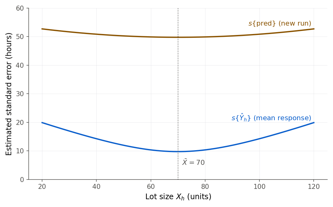
Figure 5:The mean-response standard error (blue) is smallest at the mean lot size and grows toward the extremes. The prediction standard error (yellow) stays near 49 hours everywhere, because it is dominated by a single run’s own scatter, which does not shrink no matter where you predict.
3.5 Prediction interval for a new observation
Intuition
Here is the distinction that trips up more practitioners than any other. The confidence interval of 3.4 Confidence interval for a mean response is about the average run of size . But the engineers do not schedule an average run; they schedule one specific run next week, and they want to know where its hours will land. A single run scatters around the mean by its own random error , and no amount of data removes that scatter. So predicting a single new observation carries two sources of uncertainty: our uncertainty about where the line is (the same as before), plus the new run’s own irreducible variance . The interval that accounts for both is the prediction interval (Definition 3.6), and it is always wider than the confidence interval.
The whole choice comes down to one question, and Figure 6 lays it out. Ask what you are bounding: the average outcome over many cases at , or the outcome of one specific new case. The left answer is a confidence interval; the right answer is a prediction interval. Decide the question first, and the formula follows.
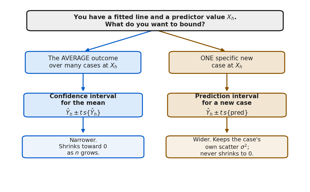
Figure 6:Pick the interval by naming the question, not by taste. Averaging over many cases at X_h calls for the confidence interval (left, narrow); planning for one new case calls for the prediction interval (right, wide). The only difference in the formula is the extra sigma-squared the new case brings.
Formula
For a new observation at , the estimated variance of the prediction error is , and the prediction interval follows.
In words: this is the mean-response variance with an extra (the leading 1) added for the new run’s own scatter. That extra term is usually the dominant one, which is why the prediction interval is much wider and why, unlike the confidence interval, it never shrinks to zero even with infinite data.
Derivation
Derivation (variance of a prediction). The quantity we bound is the prediction error , the gap between the actual new run and our forecast. The new run is , and its error is independent of the past data that produced . Two independent pieces, so their variances add:
Replacing by gives , and standardizing the prediction error by again yields a distribution. The interval follows.
The gap between the two intervals is not a modeling choice; it is a fact about the two questions, and each interval keeps its own 95% promise. We can check this by simulation, which is the surest way to see that a prediction interval really does trap a new observation 95% of the time. Figure 7 runs the experiment.
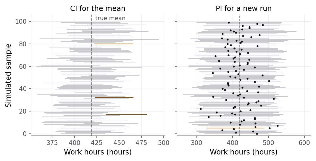
Figure 7:For 100 simulated datasets, the left panel builds a confidence interval for the mean and checks it against the fixed true mean; the right panel builds a prediction interval and checks it against a freshly drawn new run. Both catch their target about 95 times in 100, but the prediction intervals (right) are far wider because they must cover one run’s own scatter.
set.seed(4210)
b0_true <- 62.366; b1_true <- 3.5702; sigma <- 48.82
xh <- 100
mu_h <- b0_true + b1_true * xh
tcrit <- qt(0.975, n - 2)
ci_hits <- 0; pi_hits <- 0; N <- 5000
for (i in 1:N) {
  ysim <- b0_true + b1_true * x + rnorm(n, 0, sigma)
  f <- lm(ysim ~ x)
  pr <- predict(f, data.frame(x = xh), se.fit = TRUE)
  s_mean <- pr$se.fit
  s_pred <- sqrt(pr$se.fit^2 + sum(residuals(f)^2) / (n - 2))
  if (abs(pr$fit - mu_h) <= tcrit * s_mean) ci_hits <- ci_hits + 1
  ynew <- mu_h + rnorm(1, 0, sigma)
  if (abs(pr$fit - ynew) <= tcrit * s_pred) pi_hits <- pi_hits + 1
}
round(c(CI_covers_mean = ci_hits / N, PI_covers_new = pi_hits / N), 4)
CI_covers_mean PI_covers_new
0.9496 0.9458 from scipy import stats
rng = np.random.default_rng(4210)
b0_true, b1_true, sigma = 62.366, 3.5702, 48.82
xh = 100.0
mu_h = b0_true + b1_true * xh
tcrit = stats.t.ppf(0.975, n - 2)
ci_hits = pi_hits = 0
N = 5000
for _ in range(N):
ysim = b0_true + b1_true * x + rng.normal(0, sigma, size=n)
b1s = np.sum((x - x.mean()) * (ysim - ysim.mean())) / Sxx
b0s = ysim.mean() - b1s * x.mean()
yhat = b0s + b1s * xh
mse = np.sum((ysim - (b0s + b1s * x)) ** 2) / (n - 2)
s_mean = np.sqrt(mse * (1 / n + (xh - x.mean()) ** 2 / Sxx))
s_pred = np.sqrt(mse * (1 + 1 / n + (xh - x.mean()) ** 2 / Sxx))
if abs(yhat - mu_h) <= tcrit * s_mean:
ci_hits += 1
ynew = mu_h + rng.normal(0, sigma)
if abs(yhat - ynew) <= tcrit * s_pred:
pi_hits += 1
print(round(ci_hits / N, 4), round(pi_hits / N, 4))0.9492 0.9544Across 5000 simulated datasets, the confidence interval covers the true mean about 95% of the time and the prediction interval covers a fresh new run about 95% of the time. Each interval is honest about its own question. The prediction interval earns its extra width; it is not being cautious for the sake of caution.
The gap between the two intervals is easier to believe once you can open and close it yourself. The widget below puts the sample size and the prediction location under your finger, so you can find out which band answers to more data and which one does not.
What to notice. More data collapses the blue confidence band onto the line, while the amber prediction band barely flinches. Try this. Push to 200 with at 100, then walk back out to 120 and see which band cares where you stand. The formulas behind both are in 3.5 Prediction interval for a new observation.
3.6 The analysis of variance approach
Intuition
There is a second, equivalent way to see the same inference, and it scales up beautifully to the multiple regression of later chapters. The idea is bookkeeping for variation. The response values vary; some of that variation the line explains, and some it leaves as residual scatter. If we can split the total variation cleanly into an “explained” part and a “leftover” part, we can compare them, and a big explained part relative to leftover is evidence that the slope is real.
Figure 9 shows the split for a single run: the total deviation from the mean, , breaks into the part the line accounts for, , plus the residual, . Remarkably, when you square these and sum over all runs, the cross term vanishes and the totals split just as cleanly.
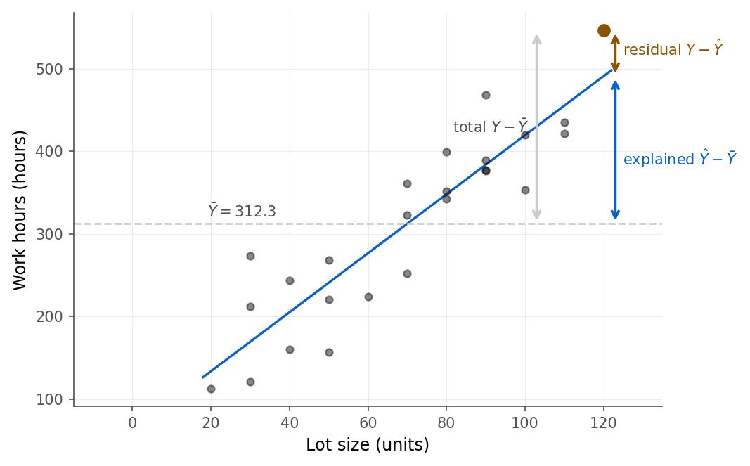
Figure 9:For one highlighted run, the total deviation from the mean (violet) equals the part the line explains (orange, mean up to the fitted line) plus the residual (red, fitted line to the point). Squaring and summing over all runs gives SSTO = SSR + SSE, because the cross term is zero.
Formula
Define the three sums of squares:
In words: the total variation of about its mean (SSTO) equals the variation the regression explains (SSR, the spread of the fitted values about the mean) plus the variation it does not (SSE, the error sum of squares from 2.4 Estimating the error variance). Each sum has degrees of freedom: for SSTO, 1 for SSR (one predictor), and for SSE. The degrees of freedom add the same way, . Dividing each sum of squares by its degrees of freedom gives a mean square (Definition 3.8).
In words: a mean square is a sum of squares averaged over its degrees of freedom, so it is a variance-like number. MSR and MSE are the two we will put in a ratio to test the slope.
Derivation
Derivation (). Split each total deviation by routing it through the fitted value:
Square both sides and sum over :
The cross term is zero. Write and expand:
Both pieces vanish by the residual identities of 2.3 Fitted values and the properties of residuals: (fitted values orthogonal to residuals) and . So the cross term is zero and . The residual identities we proved in Chapter 2 are doing the work again.
Derivation (expected mean squares). From 2.4 Estimating the error variance we already have . A similar expectation calculation, using and , gives
In words: MSE always estimates , while MSR estimates plus a term that is positive exactly when . So if the slope is zero, MSR and MSE estimate the same thing and their ratio should be near 1; if the slope is nonzero, MSR is inflated and the ratio is large. That ratio is the test.
The ANOVA table collects these quantities in a standard layout. This is the anchor later chapters extend to extra sums of squares (8.3 Extra sums of squares).
3.7 The F test and its equivalence to the t test
Intuition
The ANOVA table hands us a test almost for free. Under , both MSR and MSE estimate the same , so their ratio hovers near 1. Under , MSR is inflated by and the ratio grows. A large is evidence against the null.
But we already tested with a test in 3.2 Inference for the slope and got . Do the two tests agree? They do, exactly and always: in simple linear regression the statistic is the square of the statistic. This is worth proving, because it shows the ANOVA test is not a new test, just the test wearing different clothes.
Formula
The test of uses
and rejects when . The claimed identity is
where is the slope statistic. In words: the statistic and the squared statistic are the same number, and the tests give identical p-values.
Derivation
Derivation (). Start from the regression sum of squares. Since ,
With one regression degree of freedom, . Therefore
Now write the statistic and square it, using :
The two expressions are literally the same. Distributionally this matches a standard fact: the square of a random variable is an random variable, so squaring the slope statistic lands on the ANOVA statistic, and the critical values match too, .
Figure 10 confirms the distributional half: square 200,000 draws from a and the histogram lands on the density, with the 5% critical value 4.28 equal to 2.0692.
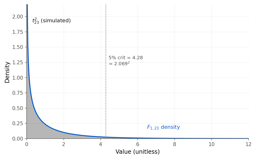
Figure 10:Squaring a t with 23 degrees of freedom produces exactly an F with 1 and 23 degrees of freedom. The 5% critical value 4.28 is the square of the t critical value 2.069, so the F test and the two-sided t test reject in identical situations.
The algebra above is three lines long, but the identity is far more convincing when you get to break the data yourself and the two numbers still refuse to disagree.
What to notice. and come off two different tables of the printout and agree to every digit shown, no matter where the points sit. Try this. Drag a point until the line flattens, then keep going until turns negative, and watch what squaring throws away. The proof is in 3.7 The F test and its equivalence to the t test.
3.8 R-squared and its interpretation
Intuition
The ANOVA split invites a natural summary: what fraction of the total variation did the line explain? That fraction is , the coefficient of determination (Definition 3.12). It runs from 0 (the line explains nothing beyond the mean) to 1 (the line passes through every point). It is the single most reported and most misread number in regression, so we will state plainly what it does and does not mean.
Formula
In words: is the proportion of the total variation in that the regression on accounts for. In simple linear regression it also equals , the square of the Pearson correlation between and , a link Chapter 4 develops (4.2 Correlation and the regression slope).
Figure 12 shows the two ingredients: the total scatter of hours about their mean (SSTO, left) shrinks to the much smaller residual scatter about the line (SSE, right). is how much of the vertical spread the line removed.
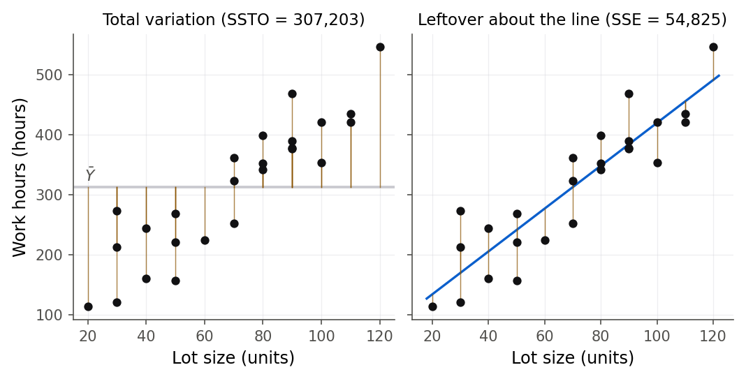
Figure 12:Left: the hours vary widely about their own mean (SSTO). Right: once lot size is in the model, the leftover scatter about the line (SSE) is much smaller. R-squared = 1 minus SSE/SSTO = 0.82 is the fraction of the vertical spread the line removed.
3.9 A confidence band for the whole line
Intuition
The confidence interval of 3.4 Confidence interval for a mean response is honest about one lot size you name in advance. But often you want to draw a band around the entire fitted line and claim, with 95% confidence, that the true line lies inside it everywhere at once. If you simply string together the pointwise intervals, the simultaneous confidence is less than 95%, because you are making many claims and some will fail by chance. The Working-Hotelling band (Definition 3.13) fixes this by using a slightly larger multiplier, so the whole-line claim holds at the stated level.
Formula
In words: the band has the same center and the same standard error as the pointwise interval, but the multiplier replaces . Because , the band is a little wider everywhere, and that extra width buys simultaneous coverage of the true line at all at once. The multiplier uses with 2 numerator degrees of freedom because the line has two parameters, and , that can both vary.
W <- sqrt(2 * qf(0.95, 2, n - 2))
round(c(W = W, t = qt(0.975, n - 2)), 4)
W t
2.6162 2.0687 W = np.sqrt(2 * stats.f.ppf(0.95, 2, n - 2))
print(round(W, 4), round(stats.t.ppf(0.975, n - 2), 4))2.6162 2.0687For Toluca the whole-line multiplier is against the pointwise , so the simultaneous band is about 26% wider than a single-point interval. Figure 13 draws both.
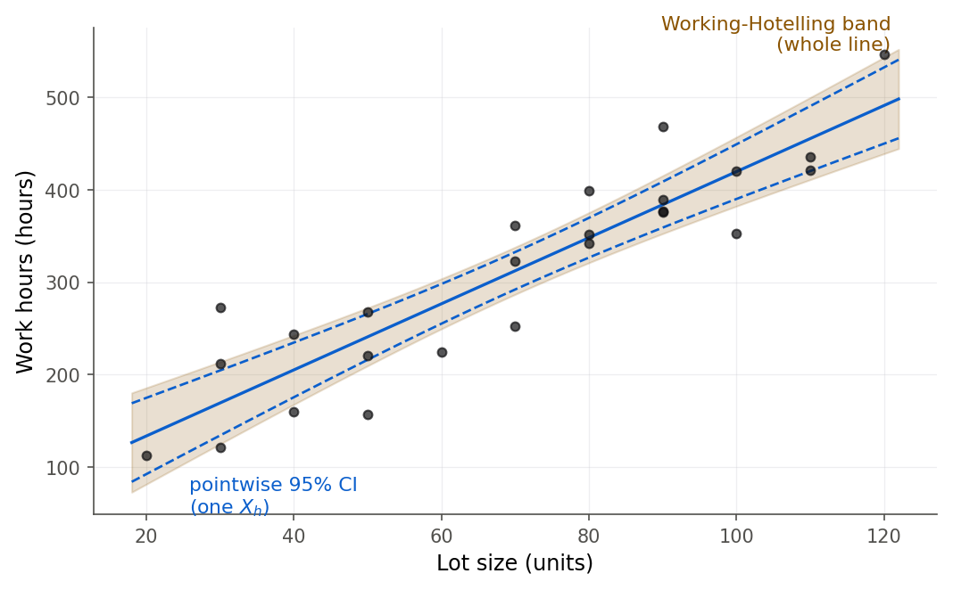
Figure 13:The pointwise confidence interval (dashed) is honest about a single chosen lot size. The Working-Hotelling band (shaded) is wider by the factor W/t = 2.62/2.07 and is honest about the entire line at once. Use the wider band when you will read the fitted line at several places.
3.10 A prediction-focused example: advertising and sales
To see the machinery on a fresh dataset, turn to the advertising data: 200 markets’ TV advertising budgets and the resulting product sales (thousands of units). A manager wants to predict sales for a new market that will receive a TV budget of 150 thousand dollars, and to understand the average effect of the budget.
Figure 14 draws both bands. Notice the prediction band comfortably contains almost all 200 markets, while the confidence band, being about the mean, does not.
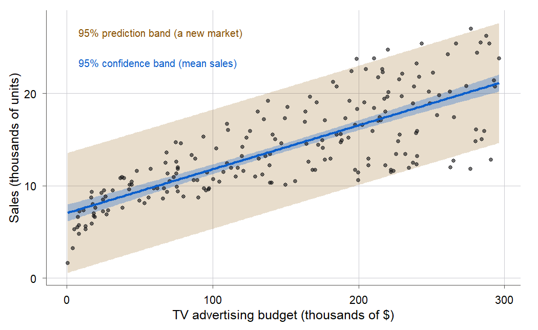
Figure 14:The advertising data with the fitted line, a narrow confidence band for mean sales (inner blue), and a wide prediction band for a single new market (outer yellow). The prediction band contains nearly all 200 markets; the confidence band is only about the average and contains few of them.
3.11 Chapter summary
You can now do inference for a simple linear regression, not just fit it. You saw why the standardized slope and intercept follow a distribution with degrees of freedom, and used it to build confidence intervals and hypothesis tests for both coefficients (the Toluca slope, , 95% CI ). You learned to tell a confidence interval for a mean response from a prediction interval for a single new observation, to derive both variance formulas, and, above all, to say which one a question needs: for a 100-unit run the mean interval is but the single-run prediction interval is . You derived the ANOVA decomposition, built the table, ran the test (), and proved it is the slope test squared. You can read correctly and widen a pointwise interval into a Working-Hotelling band () when you need the whole line.
Key results at a glance.
| Result | Statement or formula | Valid when |
|---|---|---|
| Sampling distributions of (Theorem 3.2) | , | SLR model with normal errors |
| Confidence interval for the slope (Def. 3.3) | same; test via | |
| Variance of the fitted mean (Theorem 3.5) | mean response at fixed | |
| Confidence interval for a mean response (Def. 3.4) | averaging over many cases at | |
| Variance of a prediction (Theorem 3.7) | new case’s error independent of the fit | |
| Prediction interval (Def. 3.6) | one single new observation at | |
| ANOVA decomposition (Theorem 3.9) | , df | least-squares fit with an intercept |
| Expected mean squares (Theorem 3.10) | , | SLR model |
| test and (Theorem 3.11) | , | normal errors; testing |
| Coefficient of determination (Def. 3.12) | describes variation explained, not fit correctness | |
| Working-Hotelling band (Def. 3.13) | , | simultaneous coverage of the whole line |
Key terms. Estimated standard error, confidence interval for the slope, hypothesis test for the slope, confidence interval for a mean response, prediction interval, analysis of variance, total sum of squares, regression sum of squares, mean square, test, coefficient of determination, Working-Hotelling confidence band, degrees of freedom.
You should now be able to:
Derive the sampling distributions of and and explain why inference uses .
Construct and interpret confidence intervals and hypothesis tests for the slope and intercept from software output.
Distinguish a confidence interval for a mean response from a prediction interval for a new observation, derive both, and choose the right one.
Derive the ANOVA decomposition , build the ANOVA table, and run the test for the slope.
Prove that in simple linear regression.
Interpret correctly, and name what it does and does not measure.
Construct a Working-Hotelling confidence band for the whole regression line.
Where this fits. In the workflow spine of The modeling workflow (ASK, EXPLORE, FIT, CHECK, USE), this chapter is the heart of the USE stage: it turns a fitted line into decisions and honest forecasts with stated uncertainty. Chapter 2 gave the point estimates; here we attached intervals and tests. The prediction interval (3.5 Prediction interval for a new observation) returns in Chapter 12 when we validate models on held-out data and in Chapter 15 when we forecast, where we will confront why time-ordered data makes prediction intervals harder. The ANOVA table (3.6 The analysis of variance approach) and the test (3.7 The F test and its equivalence to the t test) generalize in Chapter 8 into the extra-sums-of-squares machinery (8.3 Extra sums of squares) and the general linear test (8.4 The general linear test), which can compare whole models at once. And the tiny slope p-value here is the benchmark Chapter 5 checks against a permutation test that assumes no normality at all (5.2 The permutation test for the slope), asking whether our -based conclusion survives without the normal error model.
3.12 Frequently asked questions
Q1. What is the one-sentence difference between a confidence interval and a prediction interval? A confidence interval is for the mean response at , averaged over all cases at that predictor value; a prediction interval is for a single new case, and is wider because it must also cover that case’s own random scatter .
Q2. Why does the interval widen as moves away from ? Because the variance of the fitted mean carries a term. Away from the center, a small change in the estimated slope pivots the line a large vertical distance, so the fitted value there is less certain. Every fitted line passes through , so the uncertainty is smallest there.
Q3. Why use and not the normal distribution? Because we estimate with rather than knowing it. That extra estimation makes the reference distribution , with heavier tails than the normal. For large the two nearly coincide, but for the difference matters.
Q4. The test and the test gave the same p-value. Do I need both? In simple linear regression, no: , so they are one test. Report the test for a single slope because it keeps the direction (sign) of the effect. The test earns its keep in multiple regression, where it can test several coefficients simultaneously.
Q5. My is high. Does that mean my model is good? Not by itself. A high can accompany a curved relationship, non-constant variance, or influential outliers, all of which a residual plot would reveal. measures variation explained, not correctness, not prediction accuracy, and not causation. Read it alongside and diagnostic plots (Chapter 9).
Q6. Can I use these intervals to predict hours for a lot of 500 units? No. That is extrapolation far beyond the data range (20 to 120 units). The formulas will happily produce an interval, but its stated confidence assumes the straight-line model holds out there, which the data cannot support. Trust intervals only inside, or just barely outside, the observed range of .
Q7. What exactly does “95% confident” mean for the slope interval? It means the procedure traps the true slope in 95% of repeated samples, as Figure 15 shows with 100 simulated intervals. For your one interval , the true slope is either in it or not; the 95% describes the long-run reliability of the method, not a probability about this particular interval.
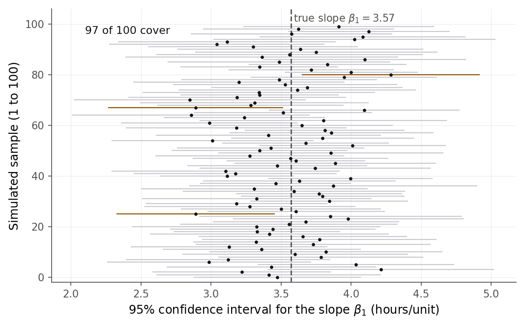
Figure 15:The meaning of 95% confidence: across 100 simulated samples, about 95 of the 95% intervals cover the true slope (blue) and a few miss (red). Any one interval either covers the truth or does not; the 95% is a property of the procedure over repeated sampling.
3.13 Practice problems
(A) In one sentence each, state what a confidence interval for the mean response and a prediction interval for a new observation are about, and say which is wider and why.
(A) The slope’s 95% confidence interval is . Explain what “95% confident” means here, and what it does not mean.
(A) Explain why the confidence interval for a mean response is narrowest at and widens on both sides.
(A) Why does inference for the slope use a distribution with degrees of freedom rather than a standard normal? Where do the degrees of freedom come from?
(A) A report states “, so the model is correct.” Give two distinct reasons this conclusion does not follow.
(A) The intercept’s 95% interval is enormously wide compared with the slope’s. Explain why, referring to where sits relative to the data.
(A) In simple linear regression the ANOVA test and the slope test always agree. State the exact relationship between the two statistics and one reason to still report the test.
(A) A colleague uses a 95% confidence interval for the mean response to budget a single upcoming production run. Explain why this understates the risk, and which interval they should use.
(B) Derive the statistic (Theorem 3.2), stating clearly which facts you take from Chapter 2, which you take on faith until Chapter 7, and why the combination is a .
(B) Derive (Theorem 3.5), including the step that and are uncorrelated.
(B) Derive the prediction-error variance (Theorem 3.7), explaining where the leading 1 comes from and why the new error is independent of .
(B) Prove the ANOVA identity (Theorem 3.9) by showing the cross term vanishes, naming the residual identities you use.
(B) Prove that in simple linear regression (Theorem 3.11), starting from .
(B) Show that (Theorem 3.10), and explain why this makes a sensible test statistic for .
(B) Show that a confidence interval for excludes 0 exactly when the two-sided test of rejects at level .
(B) Starting from and , show that , and hence that where .
(B) The Working-Hotelling multiplier is and the pointwise multiplier is . Explain, without a full proof, why must exceed and what the extra width buys.
(B) Show that the prediction interval half-width never shrinks below even as , while the confidence-interval half-width shrinks to 0. What does this say about the limits of prediction?
(C) Fit the Toluca model in R or Python. Reproduce the slope’s statistic, its p-value, and its 95% confidence interval, and confirm they match the values in this chapter.
(C) Compute a 95% confidence interval for the mean hours at units and at units. Which is wider, and does the difference match the rule?
(C) Compute both the 95% confidence interval for the mean and the 95% prediction interval for a new run at units. Report the ratio of their widths and explain it.
(C) Build the ANOVA table for Toluca in software. From it, extract , , , , and , and verify using the slope from problem 19.
(C) Using the advertising data, fit
sales ~ TV, test the slope, and give a 95% prediction interval for a new market with a TV budget of 200. Interpret the interval for a manager.(C) Write a seeded simulation (seed
4210, 2000 datasets from the fitted Toluca model at the observed lot sizes) that checks the empirical coverage of the 95% confidence interval for the mean at . Report the coverage and compare it with 0.95.(C) Reproduce the Working-Hotelling multiplier and the pointwise multiplier for Toluca. Then compute both the pointwise 95% interval and the Working-Hotelling band half-width at , and report the ratio.
(C) Regress
hours ~ lotsizeand make a plot of the fitted line with the 95% confidence band and the 95% prediction band (as in Figure 1). Describe how the two bands differ in width and shape.(B) A student claims that because is “huge,” the model must predict individual runs accurately. Explain the confusion between the test (about the slope) and prediction accuracy (about and the prediction interval), using the Toluca numbers.
(C) Using the advertising data, compute two ways: from the ANOVA sums of squares and as the square of the correlation
cor(adv$TV, adv$sales). Confirm they match, and interpret the value.
3.14 Exam practice
The problems above build skills one at a time. Exams ask you to combine them and, above all, to explain in full sentences: to read software output in context, to judge a claim, and to say what would change under a new condition. The five problems below are written in that exam voice. Work each one as if for full marks, in complete sentences, before opening the model answer. A bare number or a one-word verdict earns little credit on the real thing; the reasoning is the answer.
EP 3.1 (interpret output in context). A production scheduler has one specific new run of 80 units on next week’s calendar. Software fits the Toluca model and returns two intervals at a lot size of 80.
predict(fit, data.frame(lotsize = 80), interval = "confidence")
predict(fit, data.frame(lotsize = 80), interval = "prediction")
fit lwr upr
1 347.982 326.5449 369.4191
fit lwr upr
1 347.982 244.7333 451.2307pr = fit.get_prediction(pd.DataFrame({"lotsize": [80]}))
print("mean CI ", pr.conf_int(alpha=0.05))
print("pred PI ", pr.conf_int(obs=True, alpha=0.05))mean CI [[326.54493825 369.41910215]]
pred PI [[244.73334785 451.23069256]]Interpret each interval in one sentence, with units and in the context of this problem. Then the scheduler proposes to budget next week’s single run at “between 327 and 369 hours, 95% sure,” using the first interval. Explain in full sentences whether that is the right interval to use, which one the scheduler should use instead, and why the two intervals differ by so much.
Model answer
The first interval, hours, is a 95% confidence interval for the mean hours across all runs of 80 units: we are 95% confident that the average time for 80-unit runs, taken over many such runs, lies between about 327 and 369 hours. The second interval, hours, is a 95% prediction interval for a single new 80-unit run: we are 95% confident that one specific new run of that size will take between about 245 and 451 hours. The scheduler’s plan is wrong, and it will understate the risk. The confidence interval describes where the long-run average lands, but next week’s job is one run, not an average, and a single run carries its own random scatter of about hours on top of our uncertainty about the line. The scheduler should budget with the prediction interval, hours, which is roughly 206 hours wide against the confidence interval’s 43 hours. The two differ because the prediction interval adds the new run’s own error variance (the leading 1 in ), a term that never goes away no matter how much data we collect.
A weak answer labels the two intervals correctly but does not explain that a single run needs the prediction interval because it carries the extra scatter, and so misses why the confidence interval would blow the budget.
EP 3.2 (a student claims X, evaluate). A classmate writes: “Under the normal-error model the slope estimate is exactly normal, so a 95% confidence interval for the slope should use the standard normal multiplier 1.96.” The chapter instead uses . Explain in full sentences what is right and what is wrong in the classmate’s reasoning, what specific step forces the switch from 1.96 to 2.069, and what happens to the gap between the two multipliers as the sample size grows.
Model answer
The classmate is right that is exactly normal under the normal-error model: it is a linear combination of independent normal responses, so . If we knew the error standard deviation , then would be exactly standard normal and 1.96 would be the correct multiplier. The flaw is that we do not know . We estimate it by and divide by the estimated standard error instead. Replacing the fixed constant with the noisy estimate injects extra uncertainty, and that is exactly what turns the reference distribution from a normal into a with degrees of freedom, whose heavier tails require the larger multiplier 2.069 to still capture 95% of the distribution. As grows, estimates more and more reliably, the distribution approaches the normal, and the multiplier shrinks back toward 1.96, so the gap closes.
A weak answer just states “we use because is small” without naming the substitution of for as the reason, and so cannot explain why the gap vanishes as grows.
EP 3.3 (interpret output in context, evaluate a claim). The advertising data record TV budgets and
sales for markets. Fitting sales ~ TV gives the output below.
summary(fit_adv)$coefficients
anova(fit_adv)
c(R2 = summary(fit_adv)$r.squared, s = summary(fit_adv)$sigma)
Estimate Std. Error t value Pr(>|t|)
(Intercept) 7.032594 0.45784294 15.36028 0
TV 0.047537 0.00269061 17.66763 0
Df Sum Sq Mean Sq F value Pr(>F)
TV 1 3314.6 3314.6 312.14 < 2.2e-16
Residuals 198 2102.5 10.6
R2 s
0.6119 3.2587 print(sm.stats.anova_lm(fit_adv))
print(round(fit_adv.rsquared, 4), round(np.sqrt(fit_adv.scale), 4)) df sum_sq mean_sq F PR(>F)
TV 1.0 3314.618167 3314.618167 312.144994 1.467390e-42
Residual 198.0 2102.530583 10.618841 NaN NaN
0.6119 3.2587First, verify from the numbers that the statistic equals the square of the TV slope’s statistic, and explain in one sentence why that identity must hold here. Then a manager reads and and concludes, “the model is so significant that it will predict any one market’s sales to within a unit or two.” Explain in full sentences what the large actually establishes, what means, and which number in the output governs how far a single new market can fall from the line.
Model answer
The slope’s statistic is 17.66763, and its square is , which matches the value in the ANOVA table to the digits shown. This identity must hold because in simple linear regression : the test and the two-sided slope test are the same test, so the statistic carries no information the statistic did not. The large , like the tiny slope p-value, establishes only that the slope is far from zero relative to its standard error, that is, that TV budget is genuinely related to sales; it says nothing about how tightly the points hug the line. The value means that TV budget accounts for about 61% of the variation in sales across markets, leaving 39% to other factors, but a proportion of variation explained is not a promise of accurate individual prediction. The number that governs how far one new market can land from the line is the residual standard error thousand units, the typical size of a single market’s scatter about the line; it feeds the prediction interval, which the chapter found spans roughly thousand units at a budget of 150 (Example 3.7). So the manager’s “within a unit or two” is off by an order of magnitude: a significant, high- model can still predict a single market only loosely.
A weak answer confirms but then treats the large or the high as evidence of prediction accuracy, missing that (and the prediction interval built from it), not or , sets how far one case can miss.
EP 3.4 (what would change if). Suppose the Toluca engineers gathered far more production data at the same spread of lot sizes, so that the sample size grows very large while grows in proportion and stays near 2384. Explain in full sentences what happens, as , to (a) the width of the 95% confidence interval for the mean hours at , and (b) the width of the 95% prediction interval for a single new 100-unit run. Say why the two behave differently, and what that difference reveals about the limits of prediction.
Model answer
The confidence interval for the mean uses . As with growing in proportion, both and shrink to zero, so and the interval’s width shrink to zero: with unlimited data we can pin down the average hours at 100 units as precisely as we like, because the line itself becomes perfectly determined. The prediction interval uses . The same two terms vanish, but the leading 1 does not, so the prediction variance falls only to , and the interval’s half-width settles near hours rather than to zero. The two behave differently because the prediction interval must cover a single new run’s own random scatter , which no amount of data removes, whereas the confidence interval only chases the position of the line. The lesson is that prediction has a hard floor: even a perfectly estimated model cannot forecast one new run better than that run’s own irreducible variability allows.
A weak answer says “both intervals get narrower” without recognizing that the confidence interval goes to zero while the prediction interval stops at the irreducible floor.
EP 3.5 (interpret a figure, explain why). Figure 5 plots two estimated-standard-error curves against lot size: the mean-response standard error (blue) dips to a minimum near the mean lot size of 70 and rises toward both ends, while the prediction standard error (yellow) stays nearly flat near 49 hours across the whole range and sits above the blue curve everywhere. Explain in full sentences (a) why the blue curve is U-shaped with its lowest point at , and (b) why the yellow curve barely bends even though it lies above the blue one at every lot size.
Model answer
The blue curve tracks . The only part that depends on where you predict is , which is zero when and grows as moves away in either direction. That squared distance makes the curve U-shaped, with its minimum exactly at the mean lot size, because the fitted line is pinned down most tightly at the center of the data and a small tilt in the slope swings it more the further out you go. The yellow curve tracks , which has the same position-dependent term but adds the leading 1. That leading term contributes to the variance, far larger than the and pieces across the observed range, so the total is dominated by a constant and stays close to hours everywhere. The curve still bends upward slightly at the extremes for the same reason the blue one does, but the bend is tiny relative to the flat floor set by a single run’s own scatter.
A weak answer says the prediction curve is “just higher because prediction is wider” without identifying the leading 1 (the run’s own variance ) as the large, position-independent term that flattens the curve.
3.15 Chapter game
Resumen del capítulo (en español)
Este capítulo hace inferencia (inference) para la regresión lineal simple, continuando con los datos de la Toluca Company del Capítulo 2 (recta ajustada , ). El Capítulo 2 dio estimaciones puntuales; aquí añadimos incertidumbre en forma de intervalos y pruebas.
Bajo el modelo de errores normales, los estimadores y son exactamente normales, y al estandarizar con el error estándar estimado se obtiene una distribución t (t distribution) con grados de libertad. De ahí salen el intervalo de confianza (confidence interval) para la pendiente, , y la prueba de hipótesis (hypothesis test) de , con y valor p de : el tamaño del lote sí afecta a las horas.
La distinción central del capítulo es entre el intervalo de confianza para la respuesta media (mean response) y el intervalo de predicción (prediction interval) para una observación nueva. El primero describe el promedio de muchas corridas; el segundo suma la varianza propia de la corrida nueva y por eso es mucho más ancho. Para un lote de 100 unidades, el intervalo de la media es y el de predicción es . Una simulación con semilla confirma que cada uno cubre su objetivo cerca del 95%.
El enfoque de análisis de varianza (analysis of variance) descompone () y produce la prueba F (F test), con . Demostramos que en regresión simple : son la misma prueba. El coeficiente de determinación (coefficient of determination) es la proporción de variación explicada, no una medida de exactitud ni de causalidad. Por último, la banda de Working-Hotelling (Working-Hotelling band), con multiplicador , da confianza simultánea para toda la recta a la vez.