In 1973 two biologists, Michael Johnson and Peter Raven, published a count. For each of 30 islands in the Galapagos archipelago they recorded how many plant species grew there. Alongside each count they noted a handful of geographic facts: the island’s area, its highest elevation, its distance to the nearest neighbor, its distance to the big island of Santa Cruz, and the area of the closest adjacent island. The question was old and simple. Why do some islands hold hundreds of species and others only a dozen?
You have met this dataset twice already. In Chapter 9 it was a diagnostics cautionary tale. Fit an ordinary least-squares line, and one island, Isabela, the largest in the chain, sits so far out in predictor space that it bends the whole fit toward itself. In Chapter 10 you tried the standard remedy, transforming the response, and it helped the residual plots but never quite felt right. Something about the data resisted the linear model, and we promised you an honest answer later. Later is now.
The trouble is visible in one picture. Figure 1 plots species against island area with the least-squares line drawn through it. The fit does something impossible. Its prediction band has a single fixed width, so pushed toward small islands the band dips below zero and promises negative species counts. And one fixed width cannot fit both ends: small islands cluster tightly near zero while large islands scatter across hundreds. A species count cannot be negative, cannot be fractional, and its spread grows with its size. The linear model assumes none of that. This chapter builds the model that does.
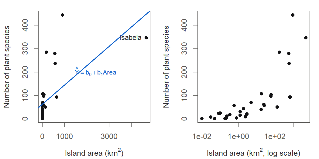
Figure 1:The Galapagos species counts against island area. Left: an ordinary least-squares line is distorted by the single huge island and assumes a constant scatter the data do not have. Right: on a log-area axis the islands spread out and the scatter clearly widens as counts grow, the signature of count data that a linear model cannot capture.
By the end of this chapter the species counts will have a model that respects what they are, the same model will handle ship-damage rates with wildly different exposures, and all of it, together with the straight lines of Chapter 2 and the logistic curves of Chapter 13, will collapse into a single family with one estimating idea. That family is the generalized linear model, and it is the payoff of this whole part of the course.
14.1 Why counts break the linear model
Intuition
A count is a whole number of things that happened: species on an island, damage incidents on a ship, customers in an hour, seizures in a week. Counts have three stubborn features. They are never negative. They are whole numbers, not fractions. And their variability grows with their average: an island that averages 5 species varies by a species or two, while an island that averages 200 varies by dozens. The linear model of Chapters 2 through 8 assumes a response that can wander anywhere on the number line, comes in any real value, and scatters by the same at every level of the predictors. Every one of those assumptions is false for a count.
The natural probability model for a count is the Poisson distribution (Definition 14.1). It describes the number of events that occur when each event is rare, events happen independently, and they arrive at a steady average rate. A Poisson distribution has a single parameter, its mean , and a notable property: its variance equals its mean. Figure 2 shows three Poisson distributions. As the mean climbs from 1 to 10, the distribution slides right, spreads out, and grows more symmetric, and at every step its spread is locked to its center.
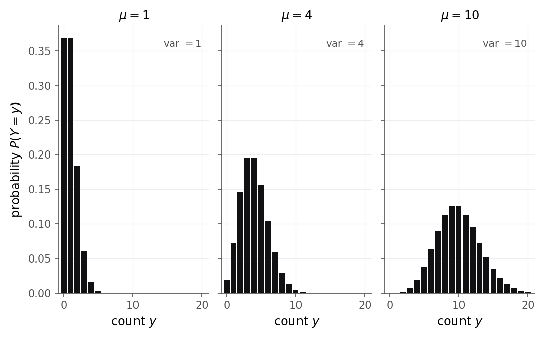
Figure 2:Three Poisson distributions. The whole distribution is set by one number, the mean, and its spread always equals that mean. Small-mean counts pile up near zero and are strongly right-skewed; large-mean counts spread wide and look nearly normal.
That mean-equals-variance link is exactly the pattern Figure 1 showed and exactly what constant-variance least squares cannot represent. Figure 3 makes the contrast explicit: the linear model draws a flat variance line, while count data ride the diagonal where variance tracks the mean.
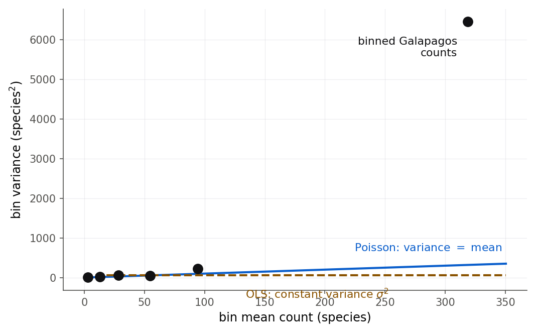
Figure 3:The assumption that fails. Ordinary least squares assumes constant variance (flat line); the Poisson model assumes variance grows with the mean (diagonal). Binned Galapagos counts climb along the diagonal, so the flat-variance model is simply the wrong shape.
Formula
A random count follows a Poisson distribution with mean when
is the count, a nonnegative whole number.
is the mean of the distribution, the average count.
is the factorial of , which normalizes the probabilities to sum to one.
In words: the probability of seeing exactly events is set entirely by the average rate . The distribution carries two facts we will use constantly,
In words: for a Poisson count the mean and the variance are the same number. This single equation is what separates count regression from everything before it, and it is the thread we follow to the end of the chapter.
Before we build a model for counts, spend a minute with the distribution itself, because the slider below is the only parameter a Poisson has.
Slide the mean count mu and watch the distribution slide right, spread out, and flatten all at once: with a Poisson you cannot move the center without moving the spread, because the variance is the mean. Back to Section 14.1.
14.2 The Poisson log-linear model and rate ratios
Intuition
We want the mean count to depend on predictors, the same ambition as ordinary regression, but with two repairs. The mean must stay positive no matter what the predictors do, and the model should describe how predictors multiply the count rather than add to it, because count processes are usually multiplicative: doubling an island’s area does not add a fixed number of species, it scales the expected number.
Both repairs come from one move: model the logarithm of the mean as a linear function of the predictors. Because the logarithm can be any real number while its inverse, the exponential, is always positive, a linear model on the log scale can range freely while the mean it produces stays positive. And because a sum on the log scale is a product on the original scale, coefficients become multipliers. Figure 5 shows the link at work: a straight line in the linear predictor becomes a curve in the mean that hugs zero for negative and climbs steeply for positive , never once dipping below zero.
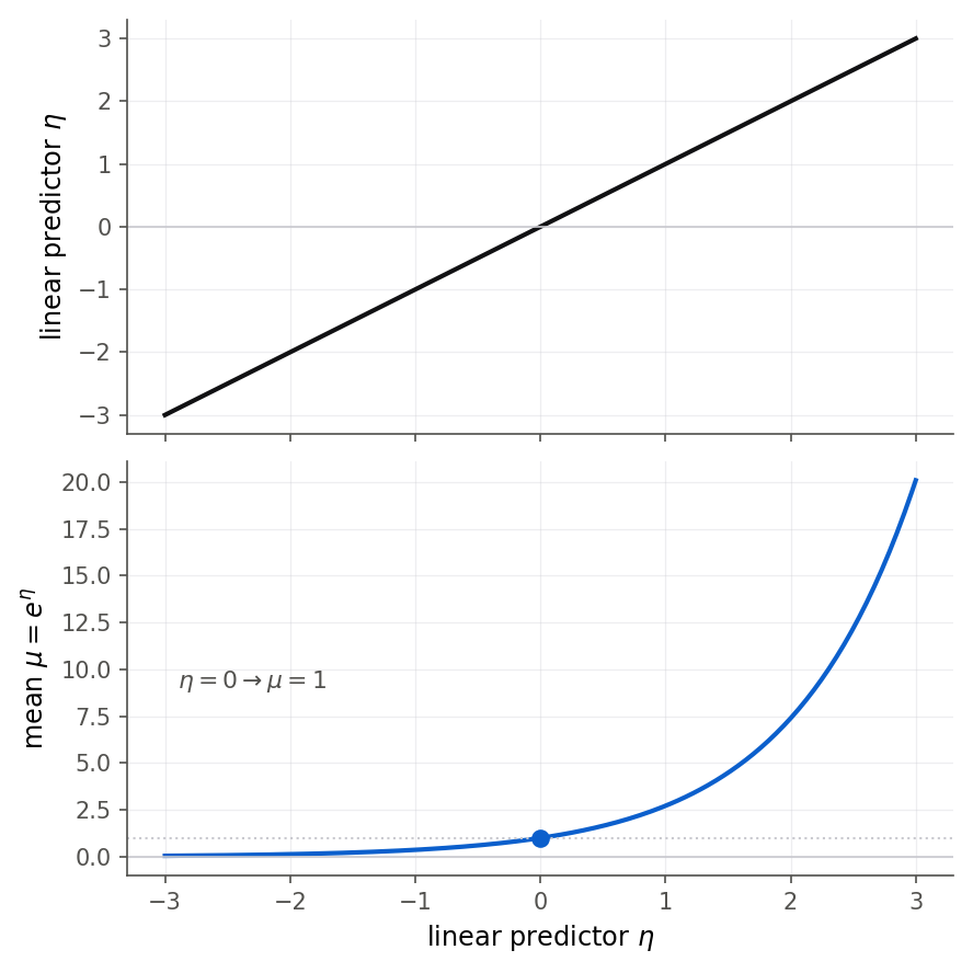
Figure 5:The log link. A straight line in the linear predictor eta (top) becomes an exponential curve in the mean mu (bottom). Because mu equals exp of eta, the mean is always positive, and equal steps in eta multiply the mean by a constant factor.
Formula
The Poisson log-linear regression model says that for each case ,
is the observed count for case , assumed Poisson given the predictors.
is its mean.
is the linear predictor, the familiar straight-line combination of predictors.
is the link function here: it maps the positive mean onto the whole real line where the linear predictor lives.
are the regression coefficients, estimated by .
Solving the link for the mean gives the multiplicative form
In words: the mean count is a product of factors, one per predictor. This is why coefficients read as rate ratios. Increase by one unit, holding the others fixed, and rises by , so is multiplied by :
In words: is the factor by which the expected count changes for a one-unit rise in . A coefficient of zero means a ratio of one, no effect; a positive coefficient means a ratio above one, the count grows; a negative coefficient means a ratio below one, the count shrinks. This is the count-data cousin of the odds ratio you met for logistic regression in 13.3 Reading coefficients as odds ratios, and of the percent-change reading of a log-scale coefficient from 10.2 The log transformation and reading its coefficients.
Here is the picture to keep in your head. On the log scale the model is an ordinary straight line, so equal steps in a predictor add the same amount each time. Exponentiate, and that even adding turns into even multiplying: each step multiplies the count by the same factor . Figure 6 shows both sides at once, using the elevation effect from the fit below, where one extra hundred meters multiplies the expected species count by about 1.42.
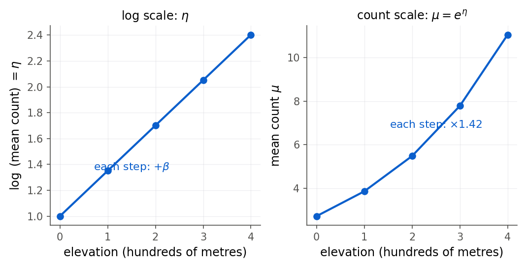
Figure 6:A coefficient is a rate ratio. On the log scale (left) each step of elevation adds the same amount to the linear predictor, a straight line. On the count scale (right) that same step multiplies the expected count by a fixed factor of about 1.42, so the count climbs faster and faster. Adding on the log scale is multiplying on the count scale.
Derivation (the Poisson log-likelihood and its score equations)
Least squares will not estimate this model: the response is not normal and the mean is not linear. As in logistic regression, we estimate by maximum likelihood, the principle from 13.2 Fitting by maximum likelihood that picks the coefficients making the observed counts most probable.
Proof. The counts are independent given the predictors, so the likelihood is the product of their Poisson probabilities, and the log-likelihood is the sum of the logs:
Substitute the model , so that , where is the predictor vector for case :
To maximize, differentiate with respect to the coefficient vector and set the result to zero. The last term does not involve . For the first two, using and ,
These are the score equations for Poisson regression. Read the first component (the one for the intercept, where has a 1): it says , the fitted means reproduce the total count. Each other component says , the residuals are orthogonal to every predictor. These are the analogues of the normal equations of 2.2 Least squares from first principles, with the fitted mean playing the role of the fitted value. The difference is that is nonlinear in the coefficients, so unlike least squares there is no closed-form solution. The equations are solved by the same iteratively reweighted least squares that fits logistic regression, sketched in 13.2 Fitting by maximum likelihood; software runs it in a handful of steps.
Notice how little changed from logistic regression. There the score equations were with a probability; here they are with a mean count. Same shape, different mean model. Section 14.6 shows this is no accident.
R
The fitting function is glm, the same one used for logistic regression, with
family = poisson. The default link for the Poisson family is the log, so you rarely name it.
gala <- read.csv("data/gala.csv")
pois_fit <- glm(Species ~ Area + Elevation + Nearest + Scruz + Adjacent,
                family = poisson, data = gala)
summary(pois_fit)
Call:
glm(formula = Species ~ Area + Elevation + Nearest + Scruz +
Adjacent, family = poisson, data = gala)
Coefficients:
Estimate Std. Error z value Pr(>|z|)
(Intercept) 3.155e+00 5.175e-02 60.963 < 2e-16 ***
Area -5.799e-04 2.627e-05 -22.074 < 2e-16 ***
Elevation 3.541e-03 8.741e-05 40.507 < 2e-16 ***
Nearest 8.826e-03 1.821e-03 4.846 1.26e-06 ***
Scruz -5.709e-03 6.256e-04 -9.126 < 2e-16 ***
Adjacent -6.630e-04 2.933e-05 -22.608 < 2e-16 ***
---
Signif. codes: 0 '***' 0.001 '**' 0.01 '*' 0.05 '.' 0.1 ' ' 1
(Dispersion parameter for poisson family taken to be 1)
Null deviance: 3510.73 on 29 degrees of freedom
Residual deviance: 716.85 on 24 degrees of freedom
AIC: 889.68
Number of Fisher Scoring iterations: 5Steering the log link by hand is the fastest way to feel what maximum likelihood is doing, so take the two coefficients yourself and let the log-likelihood tell you when you are close.
Move b0 and b1 to fit the Galapagos species counts against elevation by hand. The curve exp(b0 + b1 x) can never dip below zero, the rate ratio readout is exp(b1), the multiplier per 100 metres, and the amber band is the Poisson spread the counts are supposed to stay inside. Back to Section 14.2.
14.3 Offsets: modeling a rate instead of a count
Intuition
Raw counts are only comparable when they come from equal opportunity. A cargo ship at sea for 40,000 months has far more chance to suffer wave damage than one at sea for 100 months, so comparing their raw incident counts is meaningless. What we want is the rate: incidents per month of service. The exposure, months of service, differs from ship to ship and must be built into the model, not ignored.
The fix is elegant. Model the rate as log-linear, then rewrite it as a model for the count with one fixed piece added to the linear predictor. That fixed piece, the log of the exposure, is called an offset (Definition 14.4): a predictor whose coefficient is not estimated but pinned to one, because we know exactly how the count should scale with exposure. Double the months at sea and, all else equal, you expect double the incidents. Figure 8 shows why raw counts mislead: ship type B has by far the most incidents, but also by far the most service; per month of service its damage rate is ordinary.
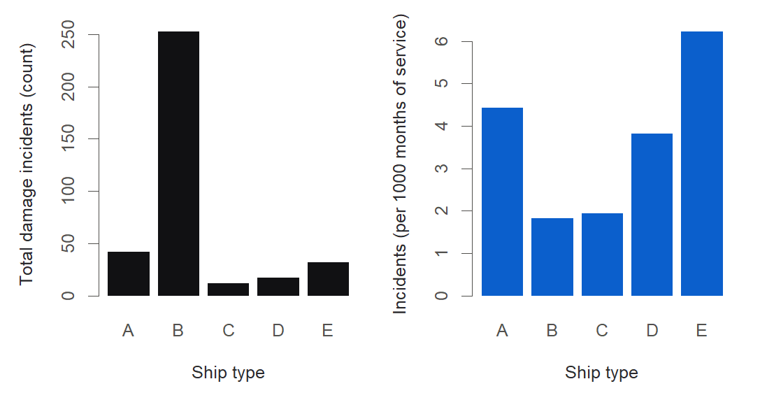
Figure 8:Why exposure matters. Left: raw damage incidents make ship type B look by far the worst. Right: once we divide by months of service to get a rate, type B is average and types A and E are the concerning ones. The offset is what lets the model compare rates instead of raw counts.
Formula
Let be the exposure for case (months of service, person-years, area surveyed) and let be the event rate per unit exposure. The count’s mean is rate times exposure, . Model the log rate as linear:
Derivation (the offset). Since , take logs:
In words: modeling the log rate is the same as modeling the log count with added to the linear predictor as a term with known coefficient exactly one. That extra term is the offset. It shifts each case’s linear predictor by its log-exposure without costing a parameter, so the estimated coefficients describe the rate , and is now a rate-ratio per unit exposure. If you wrongly dropped the offset, the model would explain incidents partly through whatever predictor happens to correlate with service time, confounding rate with exposure.
R
Ships with zero recorded service contribute no exposure and no opportunity for incidents, so
is undefined for them; we drop those rows first. The offset goes in through the
offset argument.
ships <- read.csv("data/ships.csv")
ships <- ships[ships$service > 0, ]
ships$year   <- factor(ships$year)
ships$period <- factor(ships$period)
ship_fit <- glm(incidents ~ type + year + period,
                family = poisson, offset = log(service), data = ships)
round(summary(ship_fit)$coefficients, 4)
Estimate Std. Error z value Pr(>|z|)
(Intercept) -6.4059 0.2174 -29.4600 0.0000
typeB -0.5433 0.1776 -3.0595 0.0022
typeC -0.6874 0.3290 -2.0891 0.0367
typeD -0.0760 0.2906 -0.2614 0.7938
typeE 0.3256 0.2359 1.3803 0.1675
year65 0.6971 0.1496 4.6587 0.0000
year70 0.8184 0.1698 4.8207 0.0000
year75 0.4534 0.2332 1.9446 0.0518
period75 0.3845 0.1183 3.2507 0.0012An offset is easier to believe once you have tried the alternatives, so put the exposure exponent under your finger and see what each setting is claiming about the ships.
Set the exposure exponent to 0 and the model ignores months at sea entirely, predicting the same handful of incidents for a ship at sea 45 months and one at sea 44,882. Set it to 1 and doubling the service doubles the expected count, which is exactly what the offset log t pins down. Back to Section 14.3.
14.4 Overdispersion and the quasi-Poisson fix
Intuition
The Poisson model makes a strong promise: the variance equals the mean. Real count data often break that promise by scattering more than a Poisson allows, a condition called overdispersion (Definition 14.5). Its causes are ordinary: predictors you did not measure, clustering of events, individual-to-individual differences in the underlying rate. Whatever the cause, the symptom is the same, the counts spread wider than their fitted means.
Overdispersion rarely changes the coefficient estimates much, but it wrecks their standard errors. A Poisson fit that assumes variance equals mean, when the true variance is several times larger, reports standard errors several times too small, turning noise into false significance. So overdispersion is not a nuisance to shrug off; it is the difference between an honest analysis and a misleading one. Figure 10 shows the diagnosis for the Galapagos fit: the squared residuals, which should hover around the fitted mean under a true Poisson, sit far above the variance-equals-mean line.
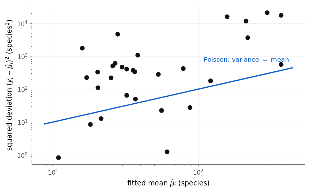
Figure 10:Diagnosing overdispersion in the Galapagos fit. Under a true Poisson the squared deviations would scatter around the diagonal (variance equals mean). Instead almost every island sits far above it, so the data vary much more than the Poisson model claims, and the model’s standard errors cannot be trusted as they stand.
Formula
Measure dispersion with the Pearson statistic (Definition 14.6) divided by its degrees of freedom. Define the Pearson residual for case and the estimated dispersion :
standardizes each residual by the Poisson standard deviation .
is the Pearson chi-square statistic.
is the residual degrees of freedom, cases minus estimated parameters.
In words: is the average squared standardized residual. Under a correct Poisson model it should be near 1. A value well above 1 signals overdispersion; a value of around 2 means the true variance is roughly twice the mean, and so on.
The quasi-Poisson fix keeps the Poisson mean model and its coefficient estimates untouched, because the score equations do not involve the variance. It only rescales the variance, assuming
for an unknown constant , estimated by . Every standard error is then multiplied by :
In words: inflate each Poisson standard error by the square root of the estimated dispersion. This is the same idea you saw in 10.4 Weighted least squares, where modeling nonconstant variance changed the weights and the standard errors while leaving the story of the mean intact. Here the variance is allowed to be a constant multiple of the mean rather than exactly the mean.
R
glm reports the raw dispersion assumption, so compute directly from the Pearson
residuals, then refit with family = quasipoisson, which does the rescaling for you.
phi_hat <- sum(residuals(pois_fit, type = "pearson")^2) / df.residual(pois_fit)
phi_hat
[1] 31.74914Figure 11 drives the point home across all five predictors: dividing each test statistic by pulls two of them below the rough significance threshold that the naive Poisson had them clearing with room to spare.
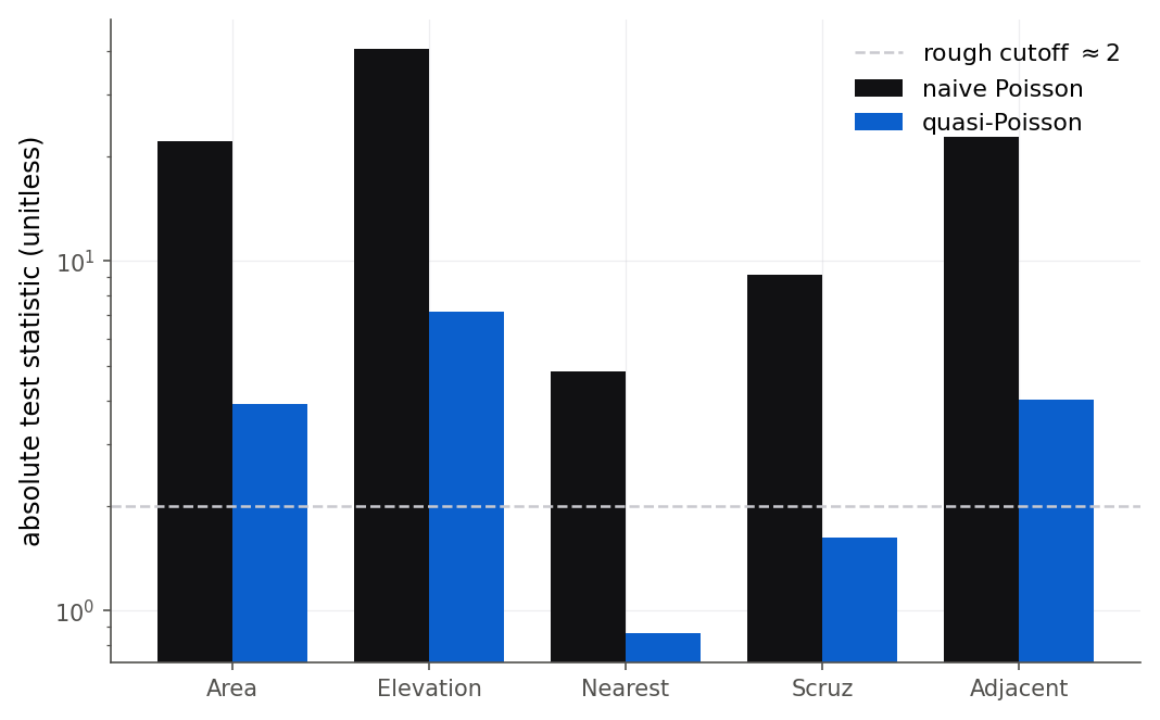
Figure 11:The cost of ignoring overdispersion. Naive Poisson test statistics (tall bars) are all far above the rough significance cutoff of 2 (dashed line). Dividing by the square root of the dispersion gives the honest quasi-Poisson statistics (short bars), and two predictors, Nearest and Scruz, drop below the cutoff.
A nod to the negative binomial
Quasi-Poisson is a quick, assumption-light patch: it does not name a probability distribution, it
just rescales variances. When you want a genuine likelihood, and therefore AIC, likelihood-ratio
tests, and honest prediction intervals, the standard choice is the negative binomial model. It
adds one parameter and lets the variance grow quadratically,
, which fits heavy overdispersion better than the
strictly linear quasi-Poisson variance. In R it is MASS::glm.nb; the Galapagos data give
, small enough to confirm severe overdispersion. For this course, diagnose with
, reach for quasi-Poisson as the everyday fix, and know the negative binomial is the next
step when you need a full likelihood.
Dispersion is just a number until you watch it move a p-value, so drag it yourself and see which Galapagos predictors survive the correction.
Raise the dispersion until the amber quasi-Poisson line finally clears the cloud of islands, somewhere near 32, and watch the test statistics for Nearest and Scruz slide under 2 as every standard error inflates by the square root of phi. Back to Section 14.4.
14.5 The Galapagos thread, resolved
We can now close the story that has run since Chapter 9. Recall the two earlier visits. Chapter 9 made the Galapagos data its lesson in influence: Isabela, the largest island, is the high-leverage point that 9.1 Leverage values and the hat matrix points to, one an ordinary least-squares fit cannot help but chase, because it sits alone at the far edge of the predictor space. In 10.2 The log transformation and reading its coefficients and 10.3 Box-Cox: letting the data choose the power you tried the classic remedy, transforming the response, taking logs or a Box-Cox power to tame the skew and the widening scatter. It improved the residual plots, but it never removed the discomfort, because the real problem was never the scale of a continuous response. The response was a count, and no transformation of a count turns it into a normal, constant-variance measurement.
The Poisson model fixes the actual defect. It builds in the nonnegativity, the multiplicative structure, and the mean-variance link that species counts genuinely have, and once we account for overdispersion its standard errors are honest. Figure 13 puts the two philosophies side by side: the log-transform-then-least-squares curve of Chapter 10, and the quasi-Poisson mean curve of this chapter, both against the raw counts on a log-area axis. They agree in the middle and part company at the extremes, where the count model keeps predictions positive and lets the scatter widen as it should.
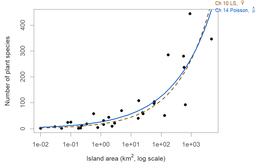
Figure 13:The resolution. The Chapter 10 transform-and-fit curve and the Chapter 14 count model agree where the data are dense and diverge at the extremes. The Poisson model is built for what the response is, a count, so it keeps predictions positive and matches the way the scatter grows with the mean.
The lesson is bigger than one archipelago. Chapter 10’s transformations are the right tool when a continuous response is on an awkward scale. When the response is a fundamentally different kind of thing, a count, a yes or no, a rate, you do not bend the response to fit the linear model; you change the model. That change is the subject of the last section, and it is the reason logistic and Poisson regression belong in the same course as least squares.
So the first decision in any analysis is not which predictors to use; it is what kind of thing the response is. Figure 14 turns that decision into a short flowchart: name the response type, follow the arrow, and you land on the matching model. The next section shows why all four destinations are really one machine.
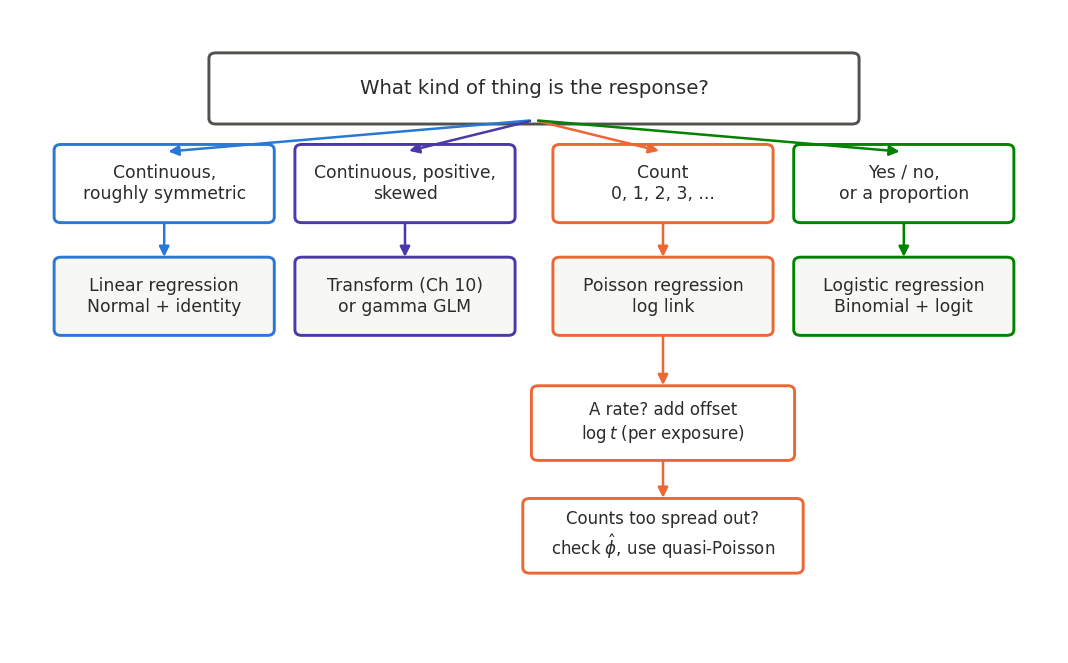
Figure 14:Diagnose the response, then pick the model. Start at the top, decide what kind of quantity the response is, and the flowchart routes you to the matching model. Counts lead to Poisson regression, with an offset when the response is really a rate and a quasi-Poisson correction when the counts are overdispersed.
14.6 One family: the generalized linear model
Intuition
Step back and look at what the last three chapters share. Ordinary regression models a continuous mean as a straight line. Logistic regression models a probability by passing a straight line through the logit link. Poisson regression models a count by passing a straight line through the log link. In every case there is a linear predictor doing the same work; what changes is only two choices: which probability distribution the response follows, and which link function connects its mean to the linear predictor. Fix those two choices and everything else, the estimation by maximum likelihood, the deviance, the workflow, is shared machinery. That is the generalized linear model, or GLM (Definition 14.8).
Formula
A generalized linear model has three parts:
The random component names the response distribution (normal, binomial, Poisson, and others), which fixes how the variance depends on the mean.
The linear predictor is the same linear combination of predictors used all book long.
The link function maps the mean onto the scale of the linear predictor; its inverse maps back, .
In words: choose a distribution and a link, and you have specified a model; the same estimation engine fits them all. The three models of this part are three rows of one table.
| Model | Response | Distribution | Link | Mean model | Chapter | |
|---|---|---|---|---|---|---|
| Linear | continuous | Normal | identity | (constant) | 2 to 8 | |
| Logistic | binary / proportion | Binomial | logit | 13 | ||
| Poisson | count | Poisson | log | 14 |
Figure 15 draws the same idea as a diagram: one linear predictor feeding three links into three response types.
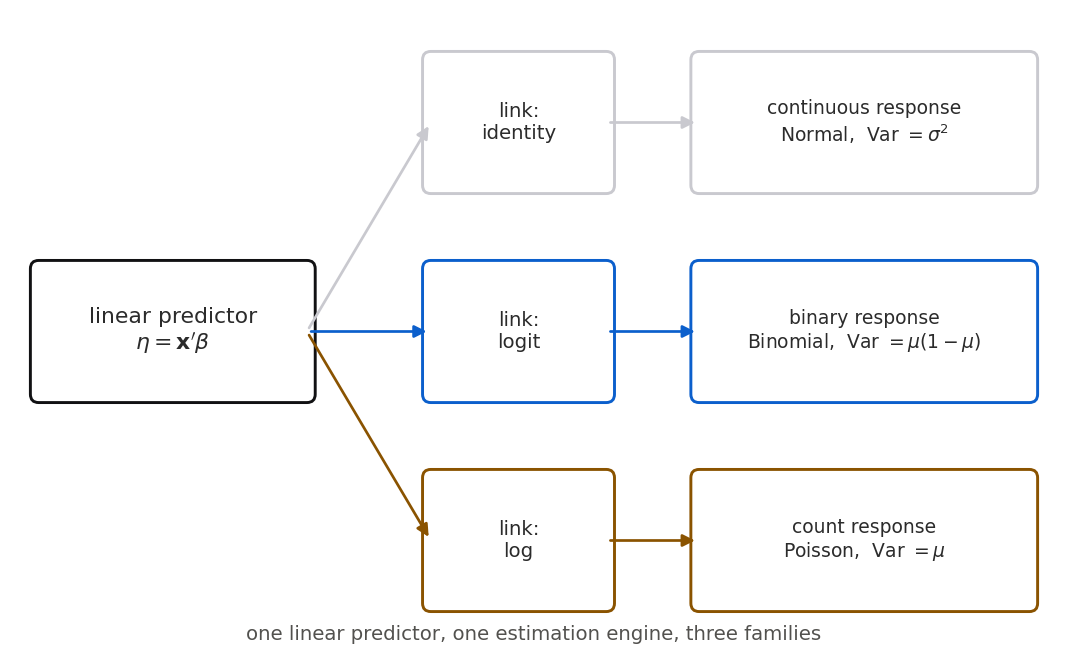
Figure 15:The generalized linear model in one picture. A single linear predictor feeds three different links to three different response types. Change the link and the family and you move between linear, logistic, and Poisson regression without changing the underlying estimation machinery.
R
The unification is not just conceptual; it is literally how the software is built. The function
glm fits every row of the table, and choosing family = gaussian(link = "identity") reproduces
ordinary least squares exactly.
14.7 Chapter summary
You can now model counts. This chapter began with why ordinary least squares is the wrong tool for a count, whose nonnegative, whole-number, mean-equals-variance behavior violates the unbounded constant-variance response the linear model assumes. The repair was the Poisson log-linear model, which models the log of the mean as a linear predictor so the fitted mean stays positive and every coefficient reads as a rate ratio . Maximizing the Poisson log-likelihood gave score equations of exactly the same form as the normal equations of Chapter 2. An offset, the log of the exposure entered with fixed coefficient one, turned the count model into a rate model for the ship data. The Pearson dispersion diagnosed the severe overdispersion in the Galapagos counts, and the quasi-Poisson correction inflated the standard errors to honest sizes while leaving the estimates alone. That finally closed the Galapagos thread from Chapters 9 and 10: the trouble was never the scale of the response, it was that the response is a count. And all of it, together with the linear and logistic models, is three rows of one generalized linear model table.
Key results at a glance
| Result | Statement or formula | Valid when |
|---|---|---|
| Poisson distribution (Def 14.1) | , | count response, rare independent events at a steady rate |
| Poisson log-linear model (Def 14.2) | , so | mean must be positive and multiplicative in predictors |
| Rate ratio | interpreting a log-linear coefficient | |
| Poisson score equations (Thm 14.3) | maximum-likelihood fit of the log-linear model | |
| Offset (Def 14.4) | modeling a rate with exposure | |
| Pearson dispersion (Def 14.6) | checking the variance-equals-mean assumption | |
| Quasi-Poisson SE (Def 14.7) | overdispersion, | |
| Generalized linear model (Def 14.8) | family link | any exponential-family response |
Key terms. Poisson distribution, Poisson log-linear regression model, linear predictor, link function, rate ratio, score equations, offset, exposure, overdispersion, Pearson dispersion, quasi-Poisson, negative binomial, generalized linear model.
You should now be able to
Explain why ordinary least squares is the wrong tool for count responses, naming the two model assumptions it violates.
State the Poisson log-linear model and interpret its coefficients as rate ratios, in the units of the problem.
Derive the Poisson log-likelihood and its score equations, and connect them to the maximum-likelihood machinery of Chapter 13.
Use an offset to model a rate, and explain why the log of exposure enters the linear predictor with a fixed coefficient of one.
Diagnose overdispersion from the Pearson dispersion and apply the quasi-Poisson correction, and say when a negative binomial model is the better fix.
Resolve the Galapagos species question with a count model, and explain why it succeeds where the transformations of Chapter 10 fell short.
Assemble the one-table GLM framework (family plus link) that contains linear, logistic, and Poisson regression as instances of a single idea.
Where this fits. In the workflow spine of The modeling workflow this chapter lives mostly in FIT and CHECK, with a strong USE payoff. The Poisson log-linear model is a FIT step for a response that the earlier chapters’ FIT tools could not handle; the overdispersion diagnosis is a CHECK step, the count-data analogue of the residual-variance checks of Chapter 9 and the variance modeling of 10.4 Weighted least squares; and reading coefficients as rate ratios is the USE step, the count cousin of the odds ratios of 13.3 Reading coefficients as odds ratios. Looking back, this chapter completes the arc that began when Chapter 13 first broke free of the normal response: logistic regression handled yes-or-no, Poisson regression handles how-many, and the GLM table shows both as extensions of the least squares you have known since Chapter 2. Looking forward, the same “choose a family and a link” habit carries into gamma models for skewed positive data, multinomial models for several categories, and the mixed and hierarchical models that a second course in regression takes up.
14.8 Frequently asked questions
Q1. Can’t I just log-transform the counts and run ordinary least squares? You can, and people did for decades, but it has real costs. Counts of zero make undefined, forcing awkward “add 0.5” patches. The back-transformed predictions describe a median, not a mean, so they do not add up correctly. And the constant-variance assumption is still wrong even after logging. Poisson regression sidesteps all three by modeling the count directly on its own terms.
Q2. Why the log link specifically? Could I use a different one? The log link is the natural choice because it makes coefficients multiplicative (rate ratios), keeps the mean positive, and is the “canonical” link that makes the Poisson math cleanest. You can use others (the identity link gives an additive count model, occasionally useful), but the log link is the default for good reasons and is what “Poisson regression” means unless stated otherwise.
Q3. My dispersion is , below 1. Is that underdispersion, and do I fix it? Values modestly below 1 are common and usually harmless; they make Poisson standard errors slightly conservative (too large), so your tests are if anything too cautious. Genuine underdispersion (from, say, counts that are more regular than random, like eggs in a full carton) exists but is rare. Worry about well above 1, not modestly below it.
Q4. Does quasi-Poisson change my coefficient estimates? No. The coefficients solve the score equations , which never mention the variance, so quasi-Poisson leaves them identical to the Poisson fit. Only the standard errors, and therefore the p-values and confidence intervals, change. That is the whole point: the estimates were fine, the uncertainty was understated.
Q5. When should I use the negative binomial instead of quasi-Poisson? Use quasi-Poisson for a fast, distribution-free correction to standard errors. Reach for the negative binomial when you need a genuine likelihood: to compare models by AIC, to run likelihood-ratio tests, or to form prediction intervals for new counts. The negative binomial also fits very heavy overdispersion better because its variance grows quadratically in the mean.
Q6. Why did dropping the zero-service ships not bias the analysis? A ship with zero months of service had no opportunity to suffer damage, so it carries no information about the damage rate, and is undefined anyway. Removing rows with zero exposure is standard and correct; you are not discarding informative data, you are discarding rows that had no exposure to model.
Q7. The Poisson and quasi-Poisson gave the same residual deviance. Shouldn’t the fix change the fit? The deviance measures how far the fitted means sit from the data, and quasi-Poisson does not move the fitted means, so the deviance is unchanged. What changes is how we judge the deviance and the coefficients against chance: quasi-Poisson divides by the dispersion, so the same deviance now tells a more cautious story.
14.9 Practice problems
(A) List the three features of count data that the ordinary linear model fails to respect, and say which model assumption each one violates.
(A) State the mean and variance of a Poisson random variable. Why does this single fact make constant-variance least squares the wrong model for counts?
(A) In a Poisson log-linear model a predictor has coefficient . State its rate ratio and interpret it in words.
(A) Explain in one or two sentences what an offset is and why its coefficient is fixed at one rather than estimated.
(A) A Poisson fit and its quasi-Poisson refit report identical coefficients but different standard errors. Explain why.
(A) Define overdispersion and name two ordinary causes of it in real count data.
(A) Give the family and link function for each GLM row: linear regression, logistic regression, Poisson regression.
(A) A colleague computes crime rates as
crimes / populationand fits ordinary least squares. Give two reasons an offset-based Poisson model is better.(A) Why can a Poisson model never predict a negative count, whatever the predictor values? Point to the piece of the model that guarantees it.
(B) Starting from the Poisson pmf , write the log-likelihood for independent counts with , and derive the score equations (Theorem 14.3).
(B) From the score equations in problem 10, show that the intercept component forces : the fitted means reproduce the total observed count.
(B) Show that the Poisson score equations have the same form as the logistic score equations of Chapter 13 and the normal equations of Chapter 2, identifying what is in each case.
(B) Derive the offset result: starting from and , show that , and explain why enters with coefficient one.
(B) Show that in a Poisson log-linear model with a single binary predictor , the coefficient equals , the log of the ratio of mean counts between the two groups. Hence is that ratio.
(B) The quasi-Poisson model assumes . Explain why this rescaling multiplies every coefficient standard error by but leaves the coefficient estimates unchanged, referring to the score equations.
(B) Write the Pearson statistic and explain why under a correct Poisson model, so that should be near 1.
(B) For two Poisson means and with exposures entered as offsets, show that the fitted rate ratio does not depend on the exposures, so the comparison is a fair per-exposure comparison.
(B) Explain why maximum likelihood, not least squares, is used to fit the Poisson model, and describe in words how iteratively reweighted least squares reaches the estimates (you may cite the Chapter 13 sketch).
(C) Fit the Poisson model
Species ~ Area + Elevation + Nearest + Scruz + Adjacenttogala.csvin R or Python. Report the coefficient onAreaand its rate ratio for a 100 km increase.(C) For the Galapagos Poisson fit, compute the Pearson dispersion from the Pearson residuals and confirm it matches the value 31.7 in the chapter. State what it says about the model.
(C) Refit the Galapagos model with
family = quasipoisson(R) or thescale="X2"option (Python). Report which predictors are significant at the 5% level under quasi-Poisson but were significant under naive Poisson, and explain the change.(C) Fit the ships damage model
incidents ~ type + year + periodwithoffset = log(service)on the positive-service rows. Report the rate ratio forperiod75and interpret it.(C) Refit the ships model without the offset (drop the
offsetargument). Compare thetypecoefficients to the offset model and explain why they change, connecting the change to the confounding of rate and exposure.(C) Compute the ships Pearson dispersion , refit as quasi-Poisson, and report how the standard error of the
typeBcoefficient changes. Is the ship data as overdispersed as the Galapagos data?(C) Fit the Toluca model
hours ~ lotsizetwo ways:lmandglmwithfamily = gaussian(link = "identity"). Show the coefficients agree, and explain what this says about the relationship between least squares and the GLM.(C) Using the Galapagos Poisson fit, predict the expected species count for an island with
Area = 40,Elevation = 200,Nearest = 1,Scruz = 30,Adjacent = 5. Do the prediction on the linear-predictor scale and then exponentiate, and confirm software gives the same number withtype = "response".(C) Fit a negative binomial model to the Galapagos data with
MASS::glm.nb(R) orstatsmodelsNegativeBinomial(Python) and report the estimated . Compare itsElevationcoefficient to the Poisson and quasi-Poisson fits.(C) Make a diagnostic plot of squared Pearson residuals against fitted means for the Galapagos Poisson fit, with the variance-equals-mean reference line, and describe what it shows about overdispersion.
(A) Chapter 10 tried log and Box-Cox transformations on the Galapagos species counts, and they helped the residual plots but never fully satisfied. Explain why the Poisson model succeeds where those transformations fell short. Name at least two specific defects of transforming a count that the count model avoids.
14.10 Exam practice
EP 14.1. Poisson regression makes two departures from ordinary least squares: it models the log of the mean rather than the mean itself, and it estimates the coefficients by maximum likelihood rather than by minimizing a sum of squares. Explain why each departure is forced on us by the nature of count data. Tie the log link to one specific property of counts, and tie the choice of maximum likelihood to another.
Model answer
The two departures answer two different failures of least squares. The log link is forced by the fact that a count mean must be positive: species, incidents, and arrivals can never average a negative number. If we modeled the mean directly as , some predictor values would push the fitted mean below zero, an impossible count. Modeling instead lets the linear predictor range over the whole real line while the mean stays strictly positive, and as a bonus it makes the coefficients multiplicative, which matches the way count processes actually scale.
Maximum likelihood is forced by a different property: the variance of a count is not constant but equals its mean, so the response is neither normal nor constant-variance. Least squares is the right estimator when errors are normal with constant variance, because under those conditions minimizing the sum of squares is the maximum-likelihood solution and is efficient by Gauss-Markov. A count breaks both conditions, so least squares loses its justification. Maximum likelihood instead uses the actual Poisson probability of the observed counts, weighting each case by how much information it carries, and it delivers the score equations that define the fit.
A weak answer names only the “counts cannot be negative” point and stops, without connecting the choice of maximum likelihood to the failure of the normal, constant-variance assumptions that make least squares optimal in the first place.
EP 14.2. A biologist fits a two-predictor Poisson model to the Galapagos data and hands you this
output. Interpret the Elevation coefficient as a rate ratio for a rise of 100 meters, say what the
exponentiated intercept means and whether it describes any real island, and state whether you would
trust the tiny standard errors as they stand.
gala <- read.csv("data/gala.csv")
f <- glm(Species ~ Elevation + Nearest, family = poisson, data = gala)
summary(f)
Coefficients:
Estimate Std. Error z value Pr(>|z|)
(Intercept) 3.574e+00 3.819e-02 93.603 < 2e-16 ***
Elevation 1.475e-03 3.341e-05 44.151 < 2e-16 ***
Nearest 6.559e-03 1.444e-03 4.541 5.59e-06 ***
(Dispersion parameter for poisson family taken to be 1)
Null deviance: 3510.7 on 29 degrees of freedom
Residual deviance: 1806.4 on 27 degrees of freedomModel answer
The elevation coefficient is 0.001475 on the log scale, so its rate ratio for a 100-meter rise is . In context: holding the distance to the nearest island fixed, each additional 100 meters of elevation multiplies the expected number of plant species by about 1.16, a 16% increase. This is a multiplier, not an additive count; it would be wrong to say “16 more species.”
The intercept is 3.574 on the log scale, so . Literally it is the expected species count for an island with elevation zero and nearest-island distance zero. No real island has zero elevation, so this is an extrapolation outside the data and should not be read as a prediction for any actual island; it is a mathematical baseline the fit passes through.
I would not trust the standard errors as printed. The values of 44 and 94 are implausibly large, and the residual deviance of 1806 on 27 degrees of freedom is far above its degrees of freedom, a clear signal of severe overdispersion (the full Galapagos fit had ). The printed standard errors assume variance equals mean; under overdispersion they are several times too small, so the significance stars cannot be believed until the dispersion is estimated and a quasi-Poisson correction is applied.
A weak answer reads the elevation effect additively or simply repeats the significance stars without noticing that the enormous values and the inflated residual deviance point to overdispersion that makes those standard errors untrustworthy.
EP 14.3. In the ships damage model, fit with an offset of , a student sees
the coefficient period75 and writes: “Ships operated in the later period suffer 0.385
more damage incidents than those in the earlier period.” Two separate things are wrong with that
sentence. Identify and correct both, then write the statement the student should have made.
Model answer
The first error is scale. The coefficient 0.385 lives on the log-of-the-mean scale, where effects are additive, but on the count scale effects are multiplicative. To interpret it you exponentiate: . So the later period does not add 0.385 incidents; it multiplies the expected count by about 1.47, a rate ratio, which is a 47% increase, not a fixed number of extra incidents.
The second error is the offset. Because the model carries as an offset, its coefficients describe a rate of damage per month of service, not a raw count of incidents. So the comparison is between damage rates per unit of exposure, not between totals; a busy ship and an idle ship at the same period have the same rate but very different raw counts. Ignoring the offset turns a statement about rates into a false statement about counts.
The correct sentence: “Holding ship type and construction year fixed, ships operating in the later period had about 47% more damage incidents per month of service than ships in the earlier period.”
A weak answer fixes only the exponentiation and reports “47% more incidents,” forgetting that the offset makes the quantity a rate per month of service rather than a raw incident count.
EP 14.4. The two fits below are the same ships model, once with the exposure offset and once
without it. The type coefficients change sharply. Explain what happens to the type B coefficient
when the offset is dropped and why, using the exposure figures, and state which of the two fits
answers the question “which ship type is the most dangerous to operate.”
ships <- read.csv("data/ships.csv"); ships <- ships[ships$service > 0, ]
with_offset <- glm(incidents ~ type + year + period, family = poisson,
                   offset = log(service), data = ships)
no_offset   <- glm(incidents ~ type + year + period, family = poisson, data = ships)
type coefficients WITH offset: typeB -0.5433 typeC -0.6874 typeD -0.0760 typeE 0.3256
type coefficients NO offset: typeB 1.7957 typeC -1.2528 typeD -0.9045 typeE -0.1463
mean months of service by type: A 1356 B 19760 C 885 D 635 E 855
total incidents by type: A 42 B 253 C 12 D 17 E 32Model answer
With the offset, typeB , so its rate ratio is : per month of
service, type B ships suffer damage at about 58% of the baseline type A rate, making them safer than
type A, not more dangerous. Drop the offset and the coefficient flips to +1.7957, a ratio of
, which makes type B look six times worse than type A.
The exposure figures explain the flip. Type B ships accumulate a mean of months of service, roughly fifteen times the type A mean of , and they rack up 253 total incidents, far more than any other type. Without the offset the model is explaining raw counts, so it credits type B with a huge coefficient simply because those ships are at sea enormously longer and therefore have more chances to be damaged. The offset divides that exposure out, converting the response into a rate per month; once exposure is accounted for, type B’s damage rate is actually below the type A baseline. Volume of incidents and rate of incidents are different questions, and the offset is what separates them.
The offset fit is the one that answers “which type is most dangerous to operate,” because danger is a rate per unit of exposure, not a raw total. By that fit type E, with the only positive coefficient, has the highest damage rate; the no-offset fit only tells you which type happened to log the most incidents, which is mostly a statement about fleet size and time at sea.
A weak answer notes the sign flip but does not connect it to type B’s very large service time, missing that the no-offset model is conflating exposure with rate.
EP 14.5. For the full five-predictor Galapagos Poisson fit the Pearson dispersion is
. (a) Explain in context what this single number says about the species counts and
about the Poisson standard errors. (b) A colleague refits the same data with a negative binomial
model and reports and an Elevation coefficient of 0.003855, against the
Poisson value 0.003541. Interpret , and explain why the two elevation coefficients are
nearly identical even though their standard errors are not.
Model answer
(a) A Poisson model promises that the variance of a count equals its mean, which would make . The value says the Galapagos species counts scatter about 32 times more widely than a Poisson allows, severe overdispersion, most likely from island features the five predictors do not capture, spatial clustering of species, and genuine island-to-island differences in the underlying colonization rate. The consequence is specific: overdispersion barely moves the coefficient estimates, but it makes the Poisson standard errors too small by a factor of about . So the naive Poisson p-values are far too optimistic, and predictors that look strongly significant may not survive an honest correction; the point estimates, though, remain trustworthy.
(b) The parameter is the negative binomial’s extra dispersion parameter, which sets the variance to . A small makes that quadratic term large, so signals heavy overdispersion and confirms the story told. The two elevation coefficients, 0.003855 and 0.003541, agree to two digits because overdispersion corrections change how the variance is modeled, not how the mean is modeled. Both fits describe essentially the same log-linear mean relationship and solve nearly the same mean-fitting equations; what the negative binomial changes is the width of the standard errors, widening them relative to the naive Poisson to reflect the true spread. The mean is stable; only the stated uncertainty moves.
A weak answer treats as evidence that the whole model is wrong and must be discarded, or reads a large as more dispersion, missing that overdispersion inflates standard errors while leaving the coefficient estimates essentially unchanged.
Chapter game
Resumen del capítulo (en español)
Este capítulo trata la regresión de Poisson (Poisson regression) para respuestas de conteo (count), usando dos conjuntos de datos: especies de plantas en 30 islas Galápagos e incidentes de daño en barcos de carga. Un conteo nunca es negativo, es entero, y su variabilidad crece con su promedio; el modelo lineal ordinario supone lo contrario, así que falla. La distribución de Poisson describe conteos con una sola cantidad, su media , y una propiedad clave: la varianza es igual a la media.
El modelo log-lineal de Poisson propone : el logaritmo de la media es lineal en los predictores, así que la media nunca es negativa y los coeficientes se interpretan de forma multiplicativa: es una razón de tasas (rate ratio), análogo a la razón de momios de la regresión logística. Estimamos por máxima verosimilitud; derivar la log-verosimilitud da las ecuaciones de puntaje , con la misma forma que las ecuaciones normales del Capítulo 2.
Para modelar una tasa en vez de un conteo crudo, agregamos el logaritmo de la exposición como desplazamiento (offset), con coeficiente fijo igual a uno. En los barcos, la exposición son los meses de servicio; el tipo B, que parecía el peor por conteo bruto, resulta promedio al ajustar por exposición.
La sobredispersión (overdispersion) ocurre cuando los conteos varían más de lo que Poisson permite. Se diagnostica con la dispersión de Pearson , que debe estar cerca de 1; en las Galápagos vale 31.7. La corrección cuasi-Poisson multiplica cada error estándar por sin cambiar los coeficientes; el binomial negativo es la alternativa con verosimilitud completa. Así resolvemos el hilo de las Galápagos de los Capítulos 9 y 10: el problema nunca fue la escala, sino que la respuesta es un conteo. Finalmente, el modelo lineal generalizado unifica todo: una distribución más una función de enlace producen la regresión lineal, la logística y la de Poisson como tres filas de una misma tabla, con un solo motor de estimación.